Tutorial

This tutorial walks through a phyddle analysis for a binary-state speciation-extinction model (BiSSE) using an R-based simulator. It assumes that you have access to the ./workspace example projects bundled with the phyddle repository.

This tutorial explains how to:

• Understand and modify the Configuration files, config.py

• Understand and modify the Simulate script, sim_bisse.R

• Run a phyddle analysis to Train a neural network

• Make a new Estimate with a trained network

• Interpret results from Plot

The Overview page provides detailed explanations for how phyddle works and how to use it responsibly. The Appendix page contains a glossary of terms and a table of all phyddle settings.

An analysis, now!

You need a result and you need it now!

This project will use R, ape, and castor to simulate training datasets. Make sure they are installed:

# install R packages
Rscript -e 'install.packages(c("ape", "castor"), repos="https://cloud.r-project.org")'

Then, to run a phyddle analysis for bisse_r using 25,000 simulated training examples, type:

# enter bisse_r project directory
cd workspace/bisse_r

# run phyddle analysis
phyddle -c config.py --end_idx 25000

# analysis runs
# ...

# view results summary
open plot/out.summary.pdf

We did it! …but, what did we do!? We need to view the config file and simulation script to understand what analysis we ran and how to interpret the results.

Project setup

A phyddle project generally needs two key files to proceed: a Configuration file to specify how to run phyddle, and a script to Simulate training examples.

The directory ./workspace/bisse_r/ contains:

• sim_bisse.R, a simulation script written in R

• config.py, a phyddle config file designed to work with sim_bisse.R

Results from each phyddle pipeline step will be stored into a directory with the corresponding name:

./simulate/    # raw data
./format/      # formatted data
./train/       # trained network
./estimate/    # estimated parameters
./plot/        # plots and summaries
./empirical/   # empirical data (optional, see below)
./log/         # log files

See Workspace for more details regarding a typical project directory structure.

Design the simulator

We begin with the simulation script because it is the foundation of a phyddle analysis. The script defines the phylogenetic scenarios that the neural network will learn to model. It also must generate output files with particular names and formats. This section provides a brief overview for how the simulation script works; the Simulate page explains requirements for the script in greater detail.

The simulation script sim_bisse.R needs to accept four command-line arguments: the output directory, the output filename prefix, the start index for the batch of simulated replicates, and the number of simulated replicates. For example, calling

Rscript sim_bisse.R ./simulate out 1000 100

expects that the script will call the command Rscript sim_bisse.R with four arguments (./simulate, out, 1000, and 100) to generate 100 simulated datasets, indexed 1000 through 1099, saving them to the directory ./simulate with the filename prefix out.

Let’s look at the source code for sim_bisse.R. You can view the full contents of the script here: https://github.com/mlandis/phyddle/blob/main/workspace/bisse_r/sim_bisse.R.

First, we load any libraries we want to use for our simulation.

library(castor)
library(ape)

Next, we read in our command-line arguments:

args        = commandArgs(trailingOnly = TRUE)
out_path    = args[1]
out_prefix  = args[2]
start_idx   = as.numeric(args[3])
batch_size  = as.numeric(args[4])
rep_idx     = start_idx:(start_idx+batch_size-1)
num_rep     = length(rep_idx)

After that, we create filenames for the output that phyddle expects:

# filesystem
tmp_fn = paste0(out_path, "/", out_prefix, ".", rep_idx)   # sim path prefix
phy_fn = paste0(tmp_fn, ".tre")               # newick file
dat_fn = paste0(tmp_fn, ".dat.csv")           # csv of data
lbl_fn = paste0(tmp_fn, ".labels.csv")        # csv of labels (e.g. params)

We then name the different model parameters and metrics we want to collect, either to estimate or to provide to the network as auxiliary data. It helps to write down what variables you want to record before writing the simulator so design the code to generate the desired output.

# label filenames
label_names = c("log10_birth_1",      # numerical, estimated
                "log10_birth_2",      # numerical, estimated
                "log10_death",        # numerical, estimated
                "log10_state_rate",   # numerical, estimated
                "log10_sample_frac",  # numerical, known
                "model_type",         # categorical, estimated
                "start_state")        # categorical, estimated

The next step is optional. We tell the simulator the number of species per tree the neural network expects, called the tree_width. Providing phyddle with properly sized trees can speed up the Simulate and Format step, when the simulator allows for downsampling (seen soon).

# set tree width
tree_width = 500

The main simulation loop then generates and saves one dataset per replicate index. Here is a simplified representation for a two-state SSE model for how the simulation loop works:

# simulate each replicate
for (i in 1:num_rep) {

    # simulate until valid example
    sim_valid = F
    while (!sim_valid) {

        # simulation conditions
        # ...

        # simulate model type
        # ...

        # simulate start state
        # ...

        # simulate model rates
        # ...

        # simulate BiSSE tree and data
        # ...

        # is simulated example valid?
        # ...

    }

    # save tree
    # ...

    # save data
    # ...

    # save labels
    # ...

}

# done!

Now we’ll look at each part of the simulation loop. First, we will define the maximum clade size and time the simulator can run. This is the stopping condition for a birth-death model. Note, we recorde the sample_frac (rho parameter) to downsample large trees to fit within tree_width. Later, during Format, we provide the value of sample_frac as auxiliary data to the neural network for training.

# simulation conditions
max_taxa = runif(1, 10, 5000)
max_time = runif(1, 1, 100)
sample_frac = 1.0
if (max_taxa > tree_width) {
    sample_frac = tree_width / max_taxa
}

Next, we simulate a start state for the BiSSE model:

# simulate model type
start_state = sample(1:2, size=1)

We also simulate a model type. Model type 0 will assume that the birth rates are equal for states 0 and 1. Model type 1 will assume that birth rates can differ between states 0 and 1.

# simulate start state
model_type = sample(0:1, size=1)

We then simulate the birth, death, and state transition rates. These values are both training labels and model parameters that we want to estimate.

# simulate model rates
if (model_type == 0) {
    birth = rep(runif(1), 2)
} else if (model_type == 1) {
    birth = runif(2)
}
death = max(birth) * rep(runif(1), 2)
Q = matrix(runif(1), nrow=2, ncol=2)
diag(Q) = -rep(Q[1,2], 2)
parameters = list(
    birth_rates=birth,
    death_rates=death,
    transition_matrix_A=Q
)

We now have all model parameters and conditions, so we simulate a phylogeny and dataset under the BiSSE model using the R package castor:

# simulate BiSSE tree and data
res_sim = simulate_dsse(
                Nstates=num_states,
                parameters=parameters,
                start_state=start_state,
                sampling_fractions=sample_frac,
                max_extant_tips=max_taxa,
                max_time=max_time,
                include_labels=T,
                no_full_extinction=T)

Valid trees must have 10 or more taxa. Smaller trees are rejected and resampled.

# check if tree is valid
num_taxa = length(res_sim$tree$tip.label)
sim_valid = (num_taxa >= 10)   # only consider trees size >= 10

Once we have valid dataset, we save the tree using the ape package:

# save tree
tree_sim = res_sim$tree
write.tree(tree_sim, file=phy_fn[i])

We also save the simulated character data to file in csv format:

# save data
state_sim = res_sim$tip_states - 1
df_state = data.frame(taxa=tree_sim$tip.label, data=state_sim)
write.csv(df_state, file=dat_fn[i], row.names=F, quote=F)

Lastly, we save the model parameters to file in csv format. This file is later parsed into “unknown” parameters to estimate vs. “known” parameters that become auxiliary data.

# save learned labels (e.g. estimated data-generating parameters)
label_sim = c( birth[1], birth[2], death[1], Q[1,2], sample_frac, model_type, start_state-1)
label_sim[1:5] = log(label_sim[1:5], base=10)
names(label_sim) = label_names
df_label = data.frame(t(label_sim))
write.csv(df_label, file=lbl_fn[i], row.names=F, quote=F)

That completes the anatomy of the simulation script. This is a fairly simple simulation script for a specific model using a specific programming language and code base (e.g. R packages). The general logic is the same for other models and simulators. Explore the workspace projects bundled with phyddle to understand how to write simulators for other models and programming languages.

Configure the pipeline

Let’s inspect important settings defined in config.py, one block at a time. You can view the contents of config.py here: https://github.com/mlandis/phyddle/blob/main/workspace/bisse_r/config.py. Some settings are omitted for brevity. Visit the Configuration page for a detailed description of the config file.

First, let’s review the project organization settings:

#-------------------------------#
# Project organization          #
#-------------------------------#
'step'    : 'SFTEP',               # Step(s) to run
'prefix'  : 'out',                 # Prefix for output for all steps
'dir'     : './',                  # Base directory for step output

The step setting runs all five pipeline steps by default (Simulate, Format, Train, Estimate, Plot). The verbose setting instructs phyddle to print useful analysis information to screen. The prefix setting causes all saved results to use the filename prefix out.` The dir setting specifies the base directory for step output subdirectories.

#-------------------------------#
# Multiprocessing               #
#-------------------------------#
'use_parallel'   : 'T',            # Use CPU multiprocessing
'use_cuda'       : 'T',            # Use GPU parallelization w/ PyTorch
'num_proc'       : -2,             # Use all but 2 CPUs for multiprocessing

The use_parallel setting lets phyddle to use multiprocessing for the Simulate, Format, Train, and Estimate steps. The num_proc setting defines how many processors parallelization may use. The use_cuda allows phyddle to use CUDA and GPU parallelization during the Train and Estimate steps.

#-------------------------------#
# Simulate Step settings        #
#-------------------------------#
'sim_command'       : 'Rscript sim_bisse.R',   # exact command string
'start_idx'         : 0,                       # first sim. replicate index
'end_idx'           : 1000,                    # last sim. replicate index
'sim_batch_size'    : 10,                      # sim. replicate batch size

The sim_command setting specifies what command to run to simulate a batch of datasets. Note, Simulate calls this script with four arguments: the step’s output directory, the step’s output filename prefix, the start index for the batch of simulated replicates, and the number of simulated replicates. The start_idx and end_idx are set to 0 and 1000, and sim_batch_size is 10. Together, this means phyddle will simulate replicates indexed 0 to 999 in batches of 10 replicates using the command stored in sim_command. Because use_parallel was previously set to T each batch of replicates will be simulated in parallel.

#-------------------------------#
# Format Step settings          #
#-------------------------------#
'num_char'          : 1,                # number of evolutionary characters
'num_states'        : 2,                # number of states per character
'min_num_taxa'      : 10,               # min number of taxa for valid sim
'max_num_taxa'      : 500,              # max number of taxa for valid sim
'tree_width'        : 500,              # tree width category used to train network
'tree_encode'       : 'extant',         # use model with serial or extant tree
'brlen_encode'      : 'height_brlen',   # how to encode phylo brlen? height_only or height_brlen
'char_encode'       : 'integer',        # how to encode discrete states? one_hot or integer
'param_est'         : {                 # model parameters to predict (labels)
                       'log10_birth_1'     : 'num',
                       'log10_birth_2'     : 'num',
                       'log10_death'       : 'num',
                       'log10_state_rate'  : 'num',
                       'model_type'        : 'cat',
                       'start_state'       : 'cat'
                      },
'param_data'        : {                 # model parameters that are known (aux. data)
                       'sample_frac'       : 'num'
                      },
'tensor_format'     : 'hdf5',           # save as compressed HDF5 or raw csv
'char_format'       : 'csv',

This block of settings defines how Format will convert raw data into tensor format. The num_char and num_states settings determine how many evolutionary characters and (for discrete-valued characters) how many states each character has. The min_num_taxa and max_num_taxa define the minimum and maximum number of taxa trees must have to be included in the formatted tensor. Trees outside this range are excluded from the formatted tensor. The tree_width setting defines the maximum number of taxa represented in the compact phylogenetic data tensor format. Trees larger than tree_width are downsampled while trees smaller than tree_width are padded with zeros to fill the tensor.

The tree_encode setting informs phyddle that we have an extant-only tree, meaning we use the CDV+S format, rather than CBLV+S format. The brlen_encode setting instructs phyddle to encode one row of node height information from the standard CDV format, plus two additional rows of branch length information for internal and terminal branches. The char_encode setting causes phyddle to use one row with integer representation for our binary character.

The param_est and param_data settings define how phyddle handles different model variables. We identify four numerical training targets in param_est and one numerical auxiliary data variable with param_data. Any parameters that are not listed in param_est or param_data are treated as unknown nuisance parameters (i.e. part of the model, but not estimated or measured).

Setting tensor_format to hdf5 means formatted output will be stored in a compressed HDF5 file. The char_format setting means phyddle expects taxon character datasets are in csv format.

#-------------------------------#
# Train Step settings           #
#-------------------------------#
'num_epochs'        : 20,               # number of training intervals (epochs)
'trn_batch_size'    : 2048,             # number of samples in each training batch
'loss_numerical'    : 'mse',            # loss function to use for numerical labels
'cpi_coverage'      : 0.80,             # coverage level for CPIs
'prop_test'         : 0.05,             # proportion of sims in test dataset
'prop_val'          : 0.05,             # proportion of sims in validation dataset
'prop_cal'          : 0.20,             # proportion of sims in CPI calibration dataset

These settings control how phyddle runs the Train step to train, calibrate, and validate the neural network. The prop_test setting determines what proportion of simulated examples are withheld from the training dataset. Train shuffles the remaining 1.0 - prop_test proportion of training examples, and sets aside prop_val of those examples for a validation dataset. Validation data are used to identify when the network becomes overtrained – i.e. network performance against the validation dataset no longer increases or worsens. and prop_cal examples for calibration.

The num_epochs setting indicates the Train step wil run for 20 training intervals, with training batches of size 2048, as specified by trn_batch_size. The loss_numerical configuration sets mean-squared error for the loss function on numerical point estimates. determines how many training intervals are used. The cpi_coverage value of 0.80 sets the coverage level for the calibrated prediction intervals (CPIs). That is, 80% of CPIs under the training dataset are expected to contain the true value of the target variable.

There are no important settings for Estimate or Plot to discuss for this beginning tutorial.

Interface the simulator

Before launching a full analysis, it is important to validate the simulator behaves as intended and is properly interfaced with phyddle.

Warning

Do not proceed with training a neural network in phyddle until the simulator has been validated.

phyddle can only check for the presence and general format of required files. phyddle does not, and cannot, verify that the simulation script is modeling the the biological system accurately.

See Safe Usage for more information.

To validate the interface, run a small batch of simulations and inspect the output. For example, to simulate 10 datasets starting at index 0, type:

Rscript sim_bisse.R ./simulate out 0 10

This command will simulate datasets 0 through 9, saving them to the directory ./simulate with the filename prefix out. Inspect the output to ensure most replicate datasets have the following files:

• out.0.tre: a newick tree file

• out.0.dat.csv: a csv file of character data

• out.0.labels.csv: a csv file of model parameters

Some replicates may not have a complete fileset if the simulator if, for example, the simulator failed to simulate a tree with 2 or more taxa.

When phyddle fails to detect any valid examples from the script, it will suggest that you debug the simulation script. In this case, the simulation script was not properly writing labels files.

▪ Simulating raw data
Simulating: 100%|█████████████████████| 1/1 [00:01<00:00,  1.32s/it]
▪ Total counts of simulated files:
  ▪ 10 phylogeny files
  ▪ 10 data files
  ▪  0 labels files

WARNING: ./simulate contains no valid simulations. Verify that simulation command:

    Rscript sim_bisse.R ./simulate out 0 1

works as intended with the provided configuration.

Again, we stress that phyddle does not and cannot verify that the simulation script generates mathematically valid datasets under the specified phylogenetic model.

Users are responsible for validating that their simulation scripts behave properly. This form of validation generally requires some knowledge of the mathematical or statistical properties of the model. Showing that the model and the simulated data have matching expected values (means, variances, etc.) is a good strategy.

For example, a Brownian motion model can be validated by showing that the expected variance-covariance structure of traits among taxa reflects shared branch lengths and the diffusion rate. Simple birth-death models can be validated by showing the process generates the expected number of taxa for a given set of rates and process start time.

Using simulator that has published validation results can help establish whether the simulator works as intended. However, such results may be for a different version of the software and for only part of the model’s parameter space. When possible, it is still best to personally validate the simulator for the specific version and part of parameter space you will use with phyddle.

Train the network

Now that we understand how the simulation script and config file work, we can train our network to make predictions about BiSSE models:

# enter bisse_r project directory
cd workspace/bisse_r

# run all phyddle steps (SFTEP) using 25,000 simulated examples
phyddle -c config.py -s SFTEP --end_idx 25000

# analysis runs
# ...

# view results summary
open plot/out.summary.pdf

To share a trained network, you need to share these files and directory structure:

./config.py                            # configuration file
./train/out.trained_model.pkl          # trained network
./train/out.train_norm.aux_data.csv    # normalization terms for aux. data
./train/out.train_norm.labels.csv      # normalization terms for labels
./train/out.cpi_adjustments.csv        # CPI adjustments from calibration
./sim_bisse.R                          # allow others to simulate (optional)

To archive and zip these files as a tarball on a Unix-based system, use the command:

# compressed archive for trained network
tar -czf phyddle_bisse_r.tar.gz config.py sim_bisse.R ./train/*norm*.csv ./train/*.pkl ./train/*cpi*.csv

Saving the entire ./train directory also works, though it will capture training logs and predictions that aren’t strictly necessary for downstream estimation tasks.

# compressed archive for trained work; has a few extra files
tar -czf phyddle_bisse_r.tar.gz config.py sim_bisse.R ./train

You can then share the tarball how you please. Transfer it from a server to your laptop, email it to a colleague, or publish it as supplemental data so others can re-use your work.

If you receive a tarball with a trained network, decompress and unarchive the files

# uncompress the tarball
tar -xzf phyddle_bisse_r.tar.gz

Make new estimates

You can use a trained network make predictions against new empirical datasets. Note, your new data must follow the same dimensionality, scale, and formatting as the training data. In general, this will be done correctly through the Format step, provided the new datasets are (for example) measured in the same units of times and record states in the same way as the simulator.

To make new estimates, create an directory for your new empirical data:

# create a new directory for empirical data
mkdir -p ./empirical

# copy your empirical dataset(s) to the new directory
cp ~/data/psychotria.tre ./emprical/out.0.tre
cp ~/data/psychotria.dat.csv ./empirical/out.0.dat.csv
cp ~/data/kadua.tre ./empirical/out.1.tre
cp ~/data/kadua.dat.csv ./empirical/out.1.dat.csv

# run Format, Estimate, and Plot the new empirical data
# ... don't reformat simulated data (if it exists)
phyddle -c config.py -s FEP --no_sim

# view results
open ./plot/out.summary.pdf

This process should be quite fast, as it requires no new simulations or training. Note, phyddle will report potential issues with the empirical analysis as text warnings in the console. In addition, confirm that the outputted plots do not contain indicators of poor training or performance. Read the Safe Usage section for more information on how to diagnose and fix typical problems that afflict phyddle analyses.

Interpret the results

In this section, we review standard phyddle plots and how to interpret them. Exactly which figures are generated depends on how phyddle was configured.

Note

We note that phyddle is designed to be easy to use. However, its misuse can easily lead to untrustworthy results. We urge users to carefully read Overview and Safe Usage to learn how to use phyddle responsibly.

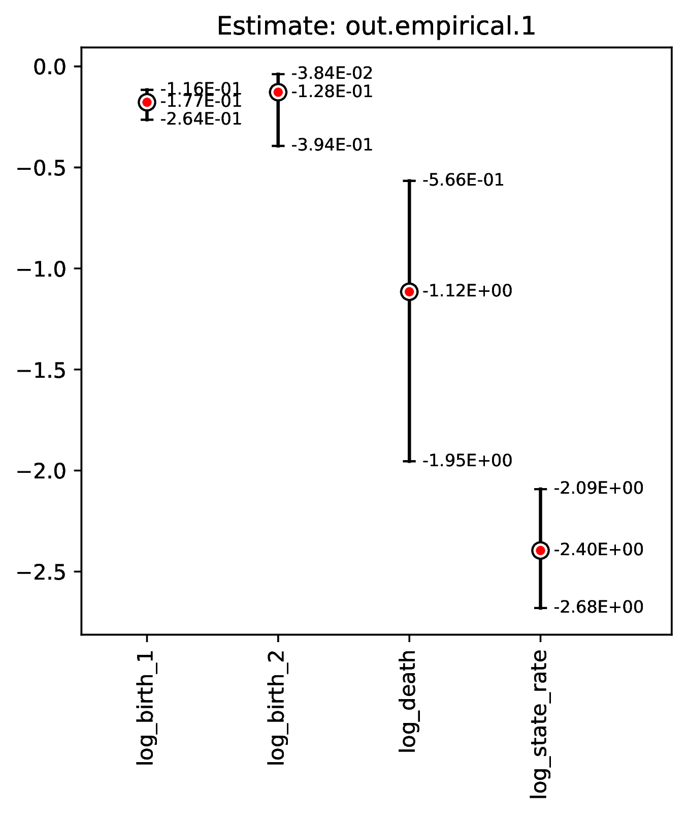
The figures named out.empirical_estimate_num_N.pdf show estimates for empirical datasets, where N represents the Nth empirical replicate. Point estimates and calibrated prediction intervals are shown for each parameter. The prediction interval represents the range of estimates that would likely contain the true model parameter value under a specified coverage level (e.g. 80% coverage means that ~80% of CPIs contain the true value).

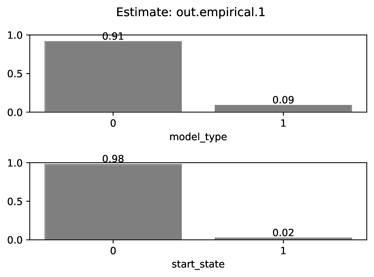
Categorical estimates for the Nth empirical datasets are shown in the figure named out.empirical_estimate_cat_N.pdf. These figures are simple bar plots reporting the probabilities across possible categories per variable. Higher probability means the network is more certain of the value of the variable.

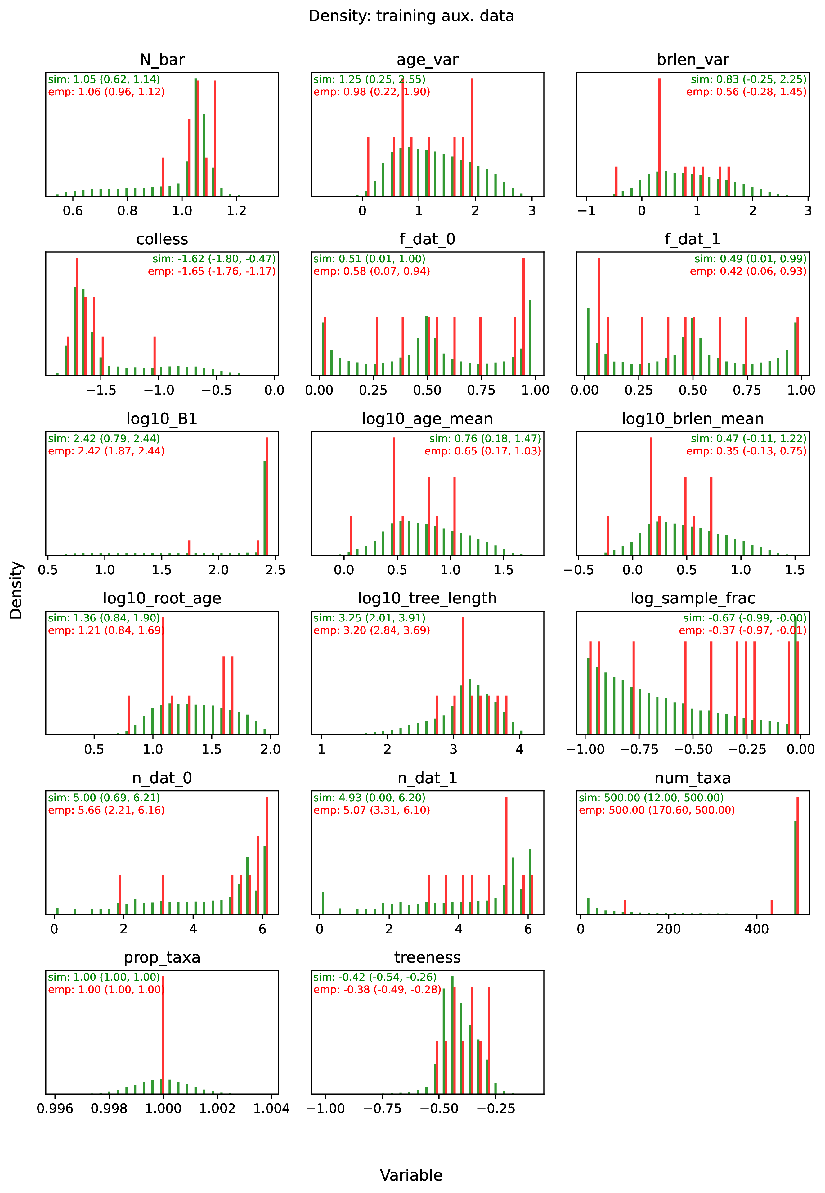
The figure out.train_density_aux_data.pdf shows the marginal density for all summary statistics generated by Format, plus the parameters defined by param_data. Green bars represent the distribution of training examples, while red bars represent empirical examples. Any empirical datasets that are outliers with respect to the training data potentially represent out-of-distribution errors that will result in untrustworthy estimates. This issue can often be repaired by simulating a training dataset that represents a wider range of evolutionary scenarios (e.g. fewer and more taxa, faster and slower rates), and then repeating the pipeline analysis. See Safe Usage for more information.

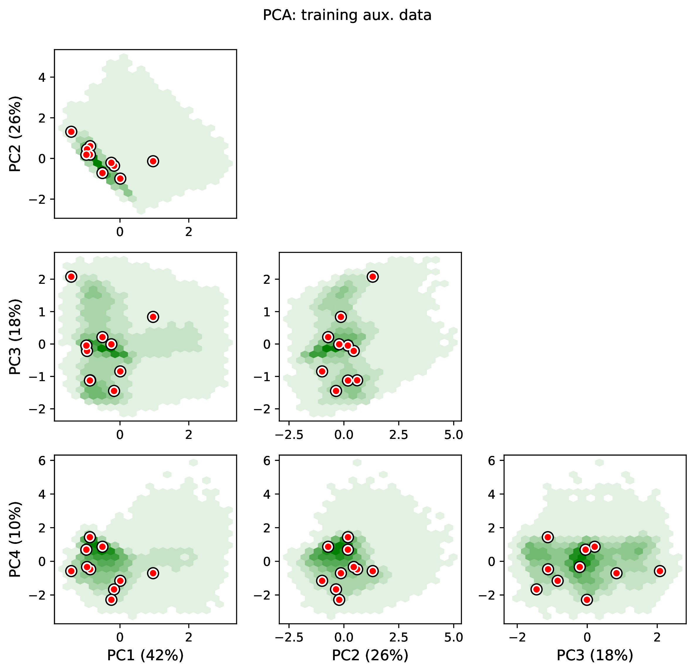
The figure out.train_pca_aux_data.pdf shows joint density of the auxiliary data as a PCA-transformed heatmap. The red dots correspond to a subsample of the empirical summary statistics to determine if they are outliers. Red dots that fall far outside the green density potentially represent out-of-distribution errors (see above).

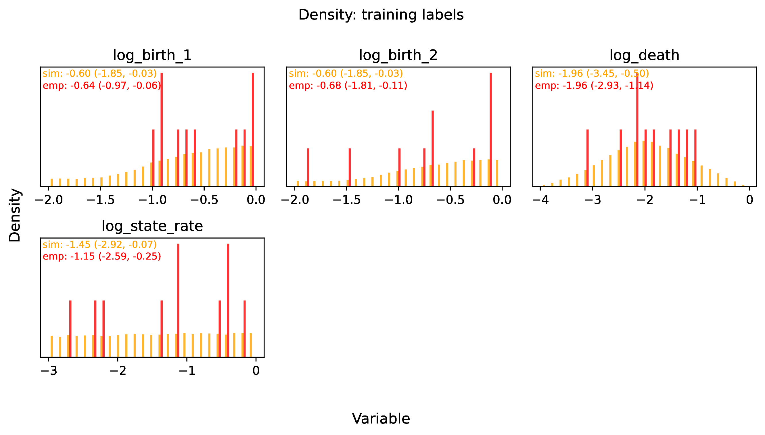
The figure out.train_density_labels_num.pdf shows the marginal density for numerical training labels defined by param_est. Orange bars represent the distribution of training examples, while red bars represent empirical examples. Any empirical estimates that are outliers with respect to the training data potentially represent out-of-distribution errors (see above).

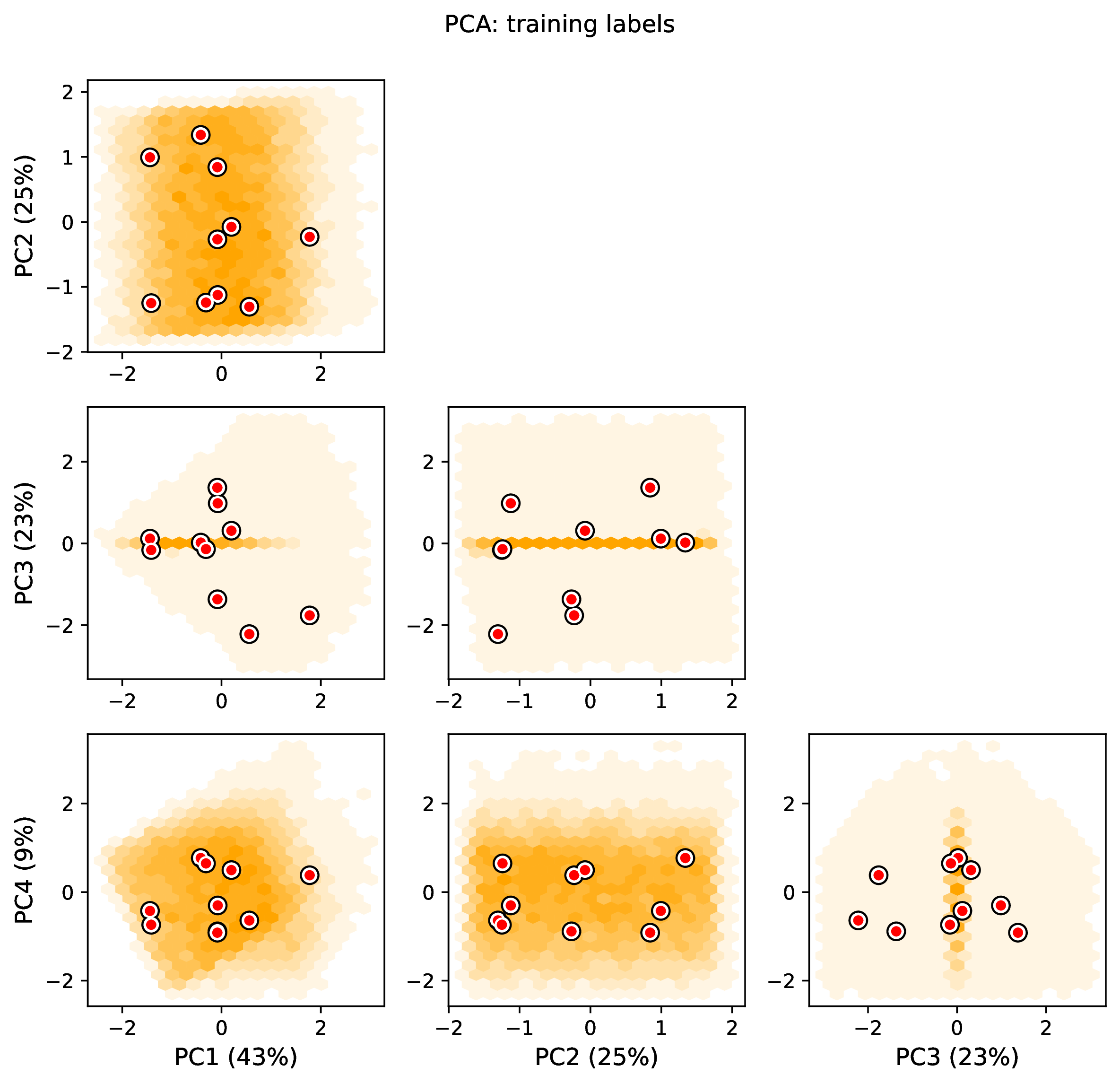
The figure out.train_pca_labels_num.pdf shows joint density of the training labels as a PCA-transformed heatmap. Red dots that fall far outside the orange density potentially represent out-of-distribution errors (see above).

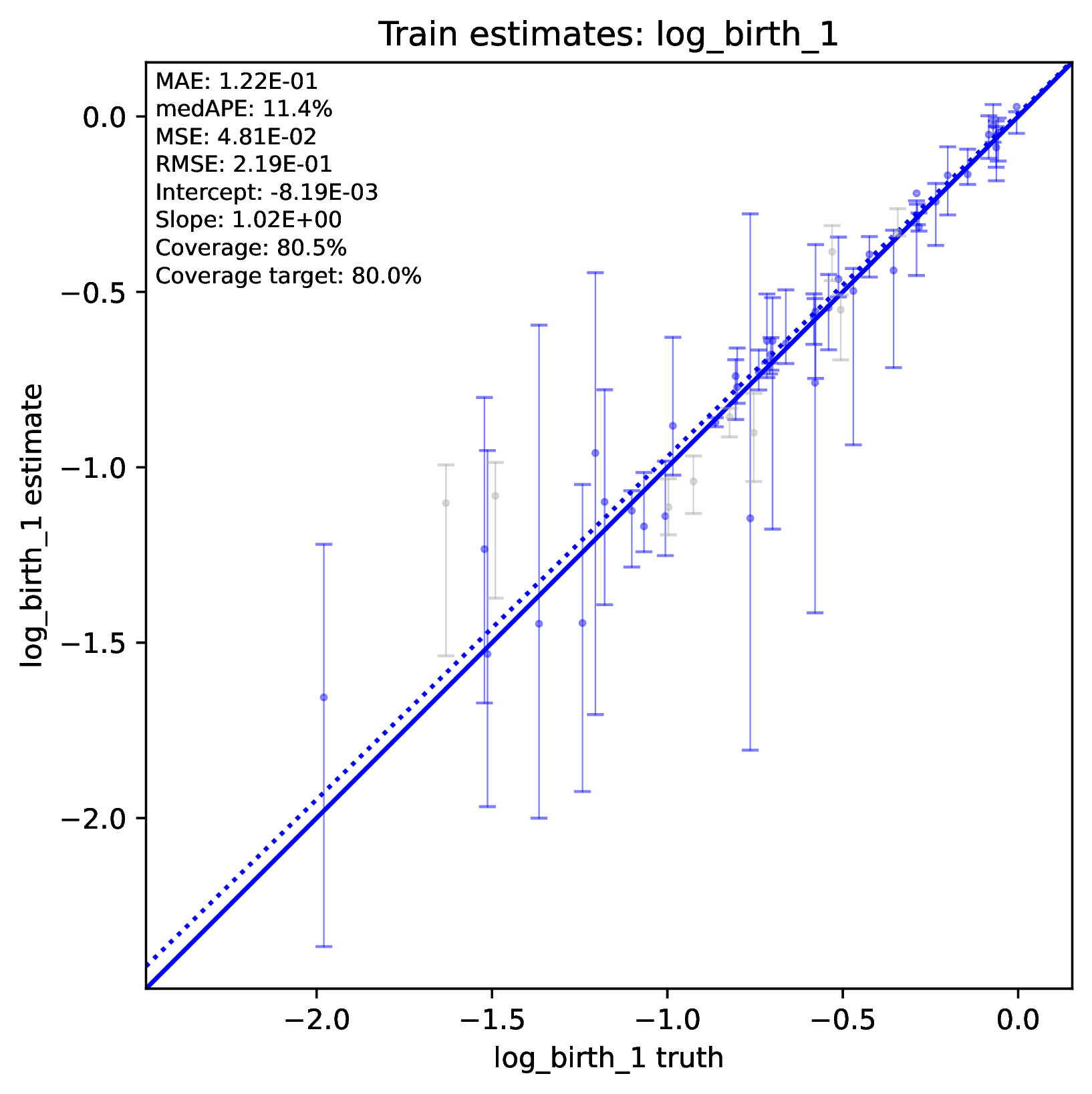
The figure out.train_estimate_log_birth_1.pdf shows trained network predictions for the training dataset. True values (x-axis) and predicted values (y-axis) should fall along the 1:1 line when accuracy is perfect. In addition, an analysis targetting 80% coverage should have roughly 80% of all intervals covering the truth (i.e. cover the 1:1 line). Performance statistics – such as mean squared error, mean absolute error, root mean squared error, median absolute percentage error, and coverage of prediction intervals – are reported in text. If performance for the training data is poor (e.g. estimated values are not correlated with the truth) then predictions from the network should not be trusted. See Safe Usage for more information.

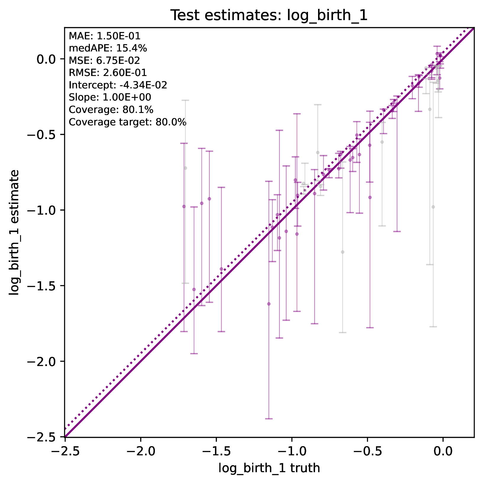
The figure out.test_estimate_log_birth_1.pdf shows trained network predictions for the test dataset (the data not used for training). The performance should be similar to those for the training data (see previous figure) if the network was trained properly. If performance is markedly worse for the test data compared to the training data, then the predictions from the network should not be trusted. See Safe Usage for more information.

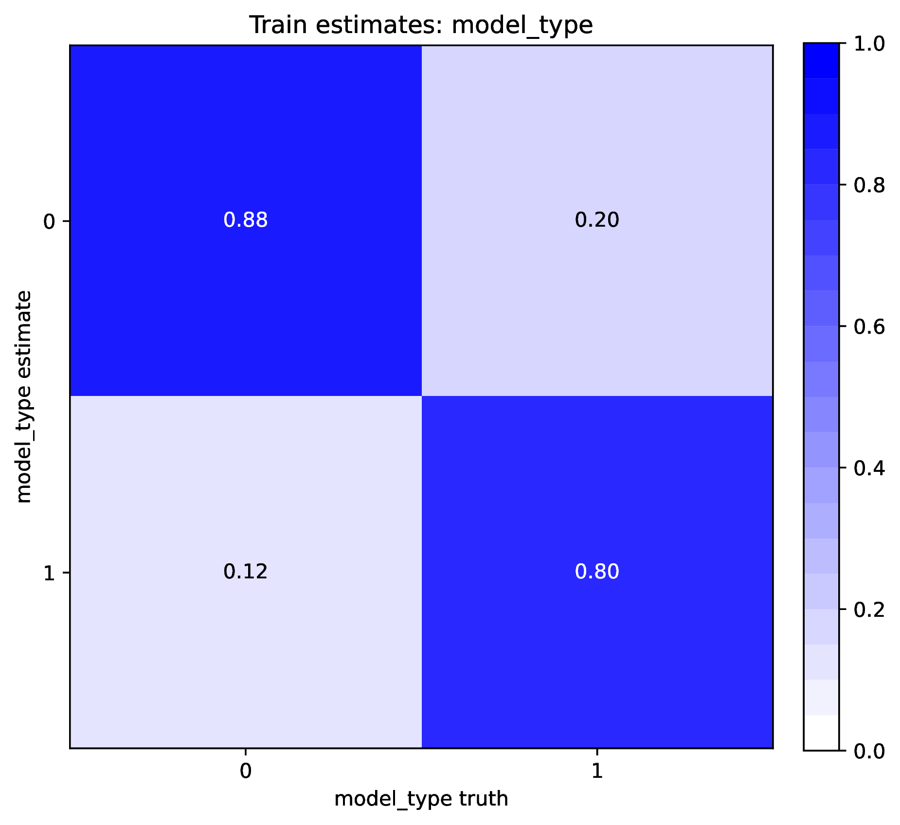
The figure out.train_estimate_model_type.png shows trained network predictions for the model type variable in the training dataset. This is a confusion matrix, comparing the truth (x-axis) to estimates (y-axis). A properly trained network that makes accurate predictions will produce a diagonal matrix, where as a poor-performing network will make off-diagonal estimates. If performance for the training data is poor (e.g. estimated values are not correlated with the truth) then predictions from the network should not be trusted. See Safe Usage for more information.

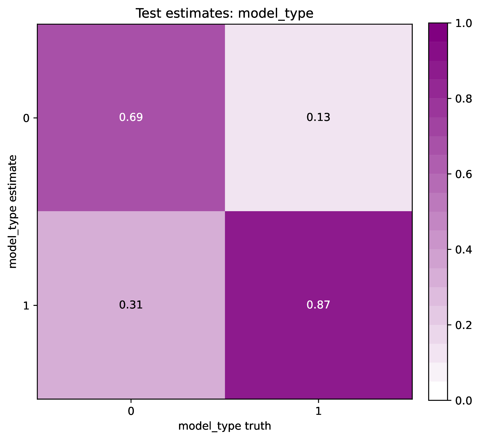
The figure out.test_estimate_model_type.png shows trained network predictions for the model type variable in the test dataset. The performance should be similar to those for the training data (see previous figure) if the network was trained properly. If performance is markedly worse for the test data compared to the training data, then the predictions from the network should not be trusted. See Safe Usage for more information.

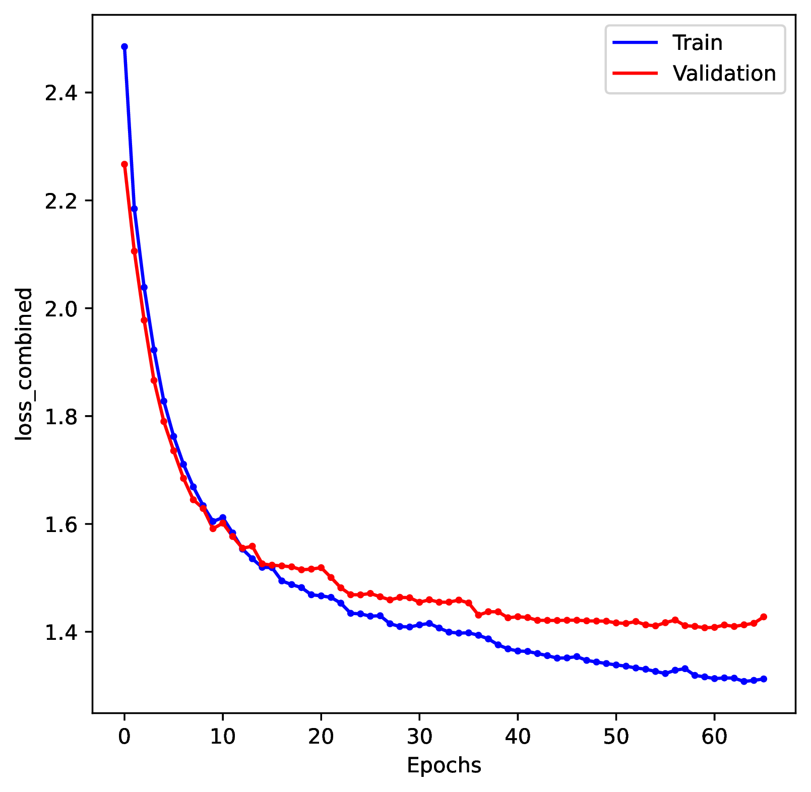
The figure out.train_history_{stat}.pdf reports how the network performed for a particular metric (y-axis) against the training dataset (blue) and the validation dataset (red) across training epochs (x-axis). The figure for loss_combined is the metric used to optimize the network. A properly trained network will show that the loss score for the training and validation datasets both decrease over time. However, even as the training dataset’s score continually decreases, the validation loss score should eventually stabilize and then slowly begin to increase. If the validation loss score never stabilizes or it increases radically, that might indicate that the network is not properly trained. See Safe Usage for more information.

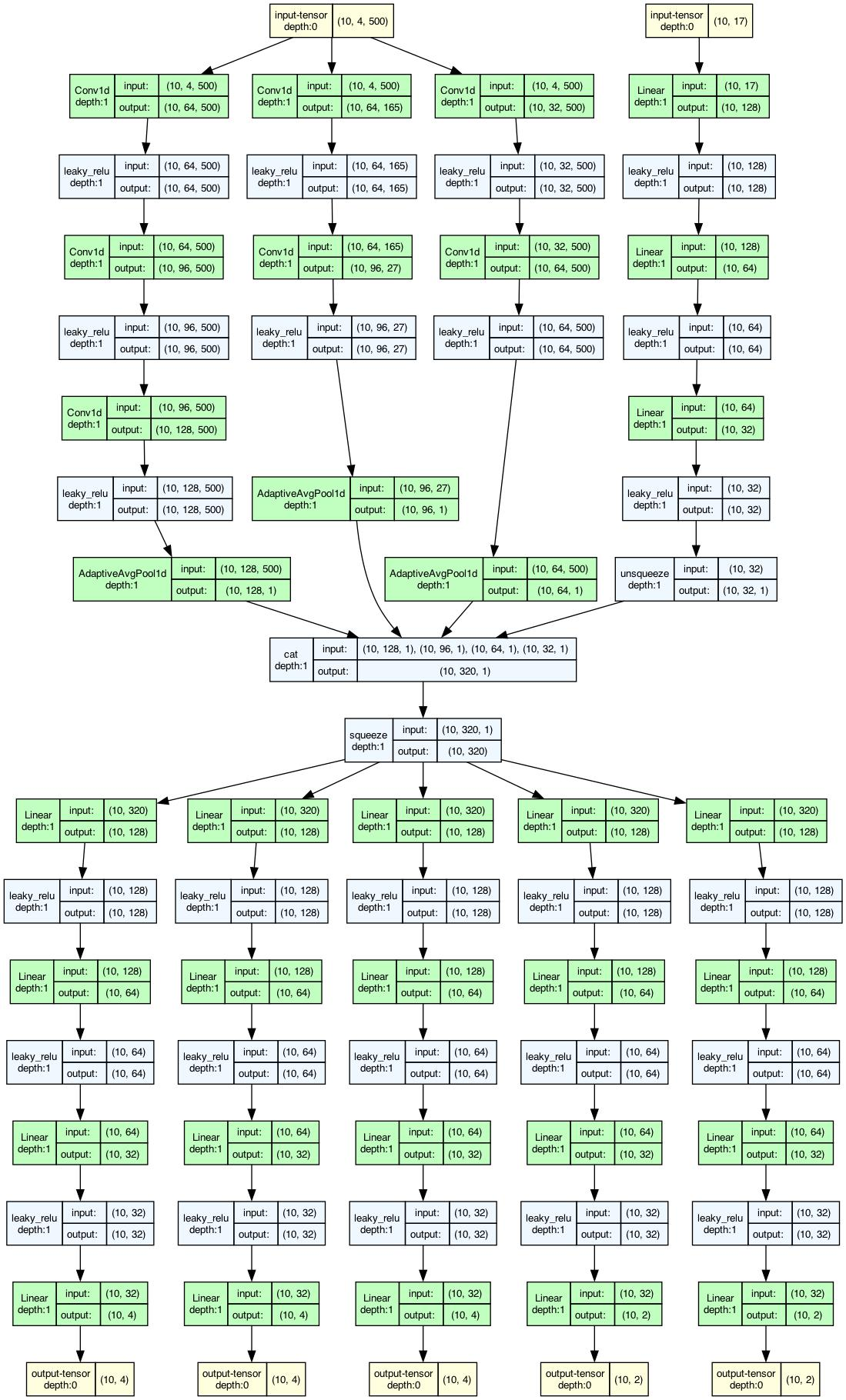
This figure out.network_architecture.pdf represents the network architecture used for training. The architecture is described in detail in Train. The numbers of layers and nodes can be modified through the Configuration file, should the user find the default architecture does not result in good performance for their modeling problem.

This concludes the tutorial! Explore the Overview documentation and other workspace project examples to learn more about phyddle’s capabilities and how to use them effectively.