Overview

Note

This page describes how a standard phyddle pipeline analysis is configured and how settings determine software behavior. Main sections: Configuration, Pipeline, Workspace, Formats, and Safe Usage. Visit Glossary to learn more about how phyddle defines different terms.

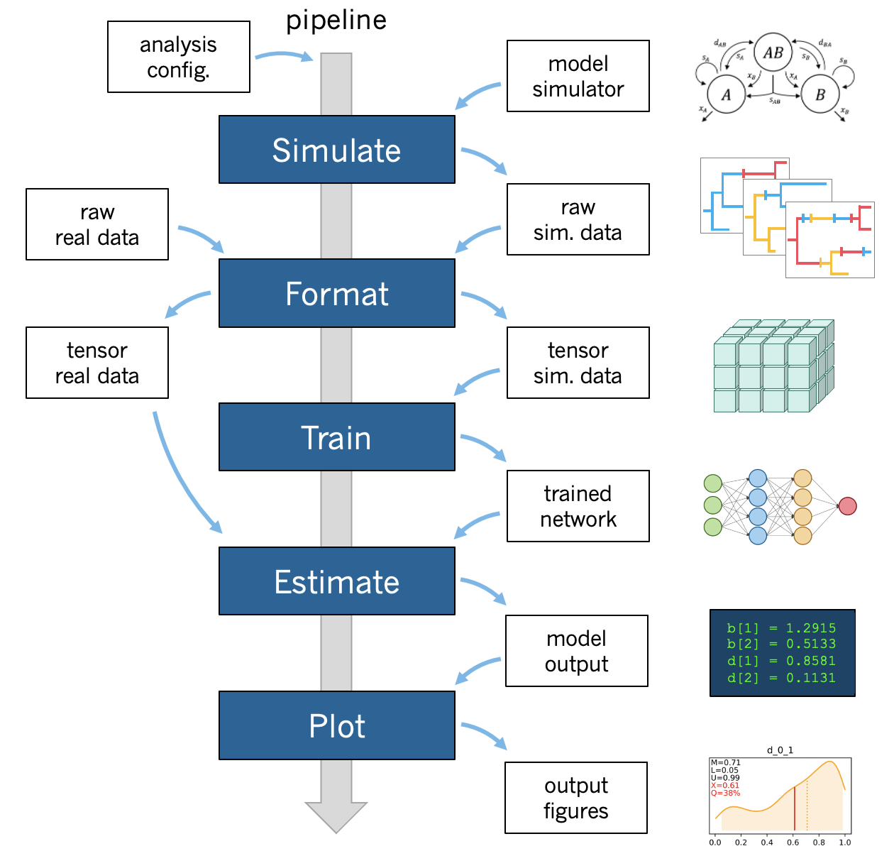
A phyddle pipeline analysis has five steps: Simulate, Format, Train, Estimate, and Plot. Standard analyses run all steps, in order, based on the analysis Configuration. Steps can also be run individually and/or multiple times under different settings and orders, which is useful for exploratory and advanced analyses.

All pipeline steps create output files, which are stored in the Workspace directories. All pipeline (except Simulate) also require input files corresponding to at least one other pipeline step. A full phyddle analysis for a project will automatically generate the input files for downstream pipeline steps and store them in a predictable project directory.

Users may also elect to use phyddle for only some steps in their analysis, and produce files for other steps by different means. For example, Format expects to format and combine large numbers of simulated datasets into tensor formats that can be used for supervised learning with neural networks. These simulated files can either be generated through phyddle with the Simulate step or outside of phyddle entirely.

Below is the standard Workspace directory structure that a standard phyddle project would use. In this section, we assume the project dir is ./workspace/example:

Simulate
- input:   None
- output:  ./workspace/example/simulate  # simulated datasets

Format
- input:   ./workspace/example/simulate  # simulated datasets
           ./workspace/example/empirical # empirical datasets
- output:  ./workspace/example/format    # formatted datasets

Train
- input:   ./workspace/example/format    # simulated training dataset
- output:  ./workspace/example/train     # trained network + train results

Estimate
- input:   ./workspace/example/format    # simulated test + empirical datasets
           ./workspace/example/train     # trained network
- output:  ./workspace/example/estimate  # test + empirical results

Plot
- input:   ./workspace/example/format    # simulated training dataset
           ./workspace/example/train     # trained network and output
           ./workspace/example/estimate  # simulated + empirical estimates
- output:  ./workspace/example/plot      # analysis figures

Configuration

There are two ways to configure the settings of a phyddle analysis: through a config file or the command line. Command line settings take precedence over config file settings.

Note

The Appendix contains a Table of Settings that summarizes all available settings.

By file

The phyddle config file is a Python dictionary of analysis arguments (args) that configure how phyddle pipeline steps behave. Because it’s a Python script, you can write code within the config file to specify your analysis, if you find that helpful. The below example defines settings into different blocks based on which pipeline step first needs a given setting. However, any setting might be used by different pipeline steps, so we concatenate all settings into a single dictionary called args, which is then used by all pipeline steps. Settings configured by file can be adjusted through the command line, if desired.

Note

By default, phyddle assumes you want to use the config file called config.py. Use a different config file by calling, e.g. phyddle --cfg my_other_config.py

Note

phyddle maintains a number of example config files for different models and simulation methods. These are organized as project subdirectories within the ./workspace directory. For example, ./workspace/bisse_r/config.py simulates under a BiSSE model with the R simulation script ./workspace/bisse_r/sim_bisse.R.

#==============================================================================#
# Config:       Example phyddle config file                                    #
# Authors:      Michael Landis and Ammon Thompson                              #
# Date:         230804                                                         #
# Description:  Simple BiSSE model                                             #
#==============================================================================#

args = {
    #-------------------------------#
    # Basic                         #
    #-------------------------------#
    'step'               : 'SFTEP',        # Pipeline step(s) defined with
                                           #   (S)imulate, (F)ormat, (T)rain,
                                           #   (E)stimate, (P)lot, or (A)ll
    'verbose'            : 'T',            # Verbose output to screen?

    #-------------------------------#
    # Analysis                      #
    #-------------------------------#
    'use_parallel'       : 'T',            # Use parallelization? (recommended)
    'num_proc'           : -2,             # Number of cores for multiprocessing
                                           #   (-N for all but N)
    'use_cuda'           : 'T',            # Use CUDA parallelization?
                                           #   (recommended; requires Nvidia GPU)

    #-------------------------------#
    # Workspace                     #
    #-------------------------------#

    'dir'                : './',           # Base directory for all step directories
    'prefix'             : 'out',                   # Prefix for all output unless step prefix given

    #-------------------------------#
    # Simulate                      #
    #-------------------------------#
    'sim_command'        : f'Rscript ./sim_bisse.R', # Simulation command to run single
                                                              #   job (see documentation)
    'sim_logging'        : 'verbose',                 # Simulation logging style
    'start_idx'          : 0,                         # Start index for simulated training replicates
    'end_idx'            : 1000,                      # End index for simulated training replicates
    'sim_batch_size'     : 10,                        # Number of replicates per simulation command

    #-------------------------------#
    # Format                        #
    #-------------------------------#
    'encode_all_sim'     : 'T',                  # Encode all simulated replicates into tensor?
    'num_char'           : 1,                    # Number of characters
    'num_states'         : 2,                    # Number of states per character
    'min_num_taxa'       : 10,                   # Minimum number of taxa allowed when formatting
    'max_num_taxa'       : 500,                  # Maximum number of taxa allowed when formatting
    'downsample_taxa'    : 'uniform',            # Downsampling strategy taxon count
    'tree_width'         : 500,                  # Width of phylo-state tensor
    'tree_encode'        : 'extant',             # Encoding strategy for tree
    'brlen_encode'       : 'height_brlen',       # Encoding strategy for branch lengths
    'char_encode'        : 'integer',            # Encoding strategy for character data
    'param_est'          : {                     # Unknown model parameters to estimate
        'log10_birth_1'      : 'num',
        'log10_birth_2'      : 'num',
        'log10_death'        : 'num',
        'log10_state_rate'   : 'num',
        'model_type'         : 'cat',
        'root_state'         : 'cat'
    ],
    'param_data'        : {                      # Known model parameters to treat as aux. data
        'sample_frac'        : 'num'
    },
    'char_format'        : 'csv',                # File format for character data
    'tensor_format'      : 'hdf5',               # File format for training example tensors

    #-------------------------------#
    # Train                         #
    #-------------------------------#
    'num_epochs'         : 20,                   # Number of training epochs
    'trn_batch_size'     : 2048,                 # Training batch sizes
    'prop_test'          : 0.05,                 # Proportion of data used as test examples
                                                 #     (to assess trained network performance)
    'prop_val'           : 0.05,                 # Proportion of data used as validation examples
                                                 #     (to diagnose network overtraining)
    'prop_cal'           : 0.2,                  # Proportion of data used as calibration examples
                                                 #     (to calibrate CPIs)
    'cpi_coverage'       : 0.95,                 # Expected coverage percent for calibrated
                                                 #     prediction intervals (CPIs)
    'cpi_asymmetric'     : 'T',                  # Use asymmetric (True) or symmetric (False)
                                                 #     adjustments for CPIs?
    'loss'               : 'mae',                # Loss function for optimization
    'optimizer'          : 'adam',               # Method used for optimizing neural network
    'phy_channel_plain'  : [64, 96, 128],        # Output channel sizes for plain convolutional
                                                 #     layers for phylogenetic state input
    'phy_channel_stride' : [64, 96],             # Output channel sizes for stride convolutional
                                                 #     layers for phylogenetic state input
    'phy_channel_dilate' : [32, 64],             # Output channel sizes for dilate convolutional
                                                 #     layers for phylogenetic state input
    'aux_channel'        : [128, 64, 32],        # Output channel sizes for dense layers for
                                                 #     auxiliary data input
    'lbl_channel'        : [128, 64, 32],        # Output channel sizes for dense layers for
                                                 #     label outputs
    'phy_kernel_plain'   : [3, 5, 7],            # Kernel sizes for plain convolutional layers
                                                 #     for phylogenetic state input
    'phy_kernel_stride'  : [7, 9],               # Kernel sizes for stride convolutional layers
                                                 #     for phylogenetic state input
    'phy_kernel_dilate'  : [3, 5],               # Kernel sizes for dilate convolutional layers
                                                 #     for phylogenetic state input
    'phy_stride_stride'  : [3, 6],               # Stride sizes for stride convolutional layers
                                                 #     for phylogenetic state input
    'phy_dilate_dilate'  : [3, 5],               # Dilation sizes for dilate convolutional layers
                                                 #     for phylogenetic state input

    #-------------------------------#
    # Estimate                      #
    #-------------------------------#
    # not currently used

    #-------------------------------#
    # Plot                          #
    #-------------------------------#
    'plot_train_color'   : 'blue',               # Plotting color for training data elements
    'plot_label_color'   : 'orange',             # Plotting color for training label elements
    'plot_test_color'    : 'purple',             # Plotting color for test data elements
    'plot_val_color'     : 'red',                # Plotting color for validation data elements
    'plot_aux_color'     : 'green',              # Plotting color for auxiliary data elements
    'plot_emp_color'     : 'black',              # Plotting color for empirical elements
    'plot_num_scatter'   : 50,                   # Number of examples in scatter plot
    'plot_min_emp'       : 5,                    # Minimum number of empirical datasets to plot densities
    'plot_num_emp'       : 10                    # Number of empirical results to plot
   }

Via command line

Settings applied through a config file can be overwritten by setting options when running phyddle from the command line. The names of settings are the same for the command line options and in the config file. Using command line options makes it easy to adjust the behavior of pipeline steps without needing to edit the config file. List all settings that can be adjusted with the command line using the --help option:

    usage: phyddle [-h] [-c] [-s] [-v] [--make_cfg ] [--save_proj ] [--load_proj ]
           [--clean_proj ] [--save_num_sim] [--save_train_fmt]
           [--output_precision] [--use_parallel] [--use_cuda] [--num_proc]
           [--no_emp] [--no_sim] [--dir] [--sim_dir] [--emp_dir]
           [--fmt_dir] [--trn_dir] [--est_dir] [--plt_dir] [--log_dir]
           [--prefix] [--sim_prefix] [--emp_prefix] [--fmt_prefix]
           [--trn_prefix] [--est_prefix] [--plt_prefix] [--sim_command]
           [--sim_logging {clean,compress,verbose}] [--start_idx]
           [--end_idx] [--sim_more] [--sim_batch_size] [--encode_all_sim]
           [--num_char] [--num_states] [--min_num_taxa] [--max_num_taxa]
           [--downsample_taxa {uniform}] [--tree_width]
           [--tree_encode {extant,serial}]
           [--brlen_encode {height_only,height_brlen}]
           [--char_encode {one_hot,integer,numeric}] [--param_est]
           [--param_data] [--char_format {csv,nexus}]
           [--tensor_format {csv,hdf5}] [--save_phyenc_csv] [--num_epochs]
           [--num_early_stop] [--trn_batch_size] [--prop_test]
           [--prop_val] [--prop_cal] [--cpi_coverage] [--cpi_asymmetric]
           [--loss_numerical {mse,mae}] [--optimizer {adam}]
           [--log_offset] [--phy_channel_plain] [--phy_channel_stride]
           [--phy_channel_dilate] [--aux_channel] [--lbl_channel]
           [--phy_kernel_plain] [--phy_kernel_stride]
           [--phy_kernel_dilate] [--phy_stride_stride]
           [--phy_dilate_dilate] [--plot_train_color] [--plot_test_color]
           [--plot_val_color] [--plot_label_color] [--plot_aux_color]
           [--plot_emp_color] [--plot_num_scatter] [--plot_min_emp]
           [--plot_num_emp] [--plot_pca_noise]

Software to fiddle around with deep learning for phylogenetic models

options:
  -h, --help            show this help message and exit
  -c, --cfg             Config file name
  -s, --step            Pipeline step(s) defined with (S)imulate, (F)ormat,
                        (T)rain, (E)stimate, (P)lot, or (A)ll
  -v, --verbose         Verbose output to screen?
  --make_cfg            Write default config file
  --save_proj           Save and zip a project for sharing
  --load_proj           Unzip a shared project
  --clean_proj          Remove step directories for a project
  --save_num_sim        Number of simulated examples to save with --save_proj
  --save_train_fmt      Save formatted training examples with --save_proj?
                        (not recommended)
  --output_precision    Number of digits (precision) for numbers in output
                        files
  --use_parallel        Use parallelization? (recommended)
  --use_cuda            Use CUDA parallelization? (recommended; requires
                        Nvidia GPU)
  --num_proc            Number of cores for multiprocessing (-N for all but N)
  --no_emp              Disable Format/Estimate steps for empirical data?
  --no_sim              Disable Format/Estimate steps for simulated data?
  --dir                 Parent directory for all step directories unless step
                        directory given
  --sim_dir             Directory for raw simulated data
  --emp_dir             Directory for raw empirical data
  --fmt_dir             Directory for tensor-formatted data
  --trn_dir             Directory for trained networks and training output
  --est_dir             Directory for new datasets and estimates
  --plt_dir             Directory for plotted results
  --log_dir             Directory for logs of analysis metadata
  --prefix              Prefix for all output unless step prefix given
  --sim_prefix          Prefix for raw simulated data
  --emp_prefix          Prefix for raw empirical data
  --fmt_prefix          Prefix for tensor-formatted data
  --trn_prefix          Prefix for trained networks and training output
  --est_prefix          Prefix for estimate results
  --plt_prefix          Prefix for plotted results
  --sim_command         Simulation command to run single job (see documentation)
  --sim_logging {clean,compress,verbose}
                        Simulation logging style
  --start_idx           Start replicate index for simulated training dataset
  --end_idx             End replicate index for simulated training dataset
  --sim_more            Add more simulations with auto-generated indices
  --sim_batch_size      Number of replicates per simulation command
  --encode_all_sim      Encode all simulated replicates into tensor?
  --num_char            Number of characters
  --num_states          Number of states per character
  --min_num_taxa        Minimum number of taxa allowed when formatting
  --max_num_taxa        Maximum number of taxa allowed when formatting
  --downsample_taxa {uniform}
                        Downsampling strategy taxon count
  --tree_width          Width of phylo-state tensor
  --tree_encode {extant,serial}
                        Encoding strategy for tree
  --brlen_encode {height_only,height_brlen}
                        Encoding strategy for branch lengths
  --char_encode {one_hot,integer,numeric}
                        Encoding strategy for character data
  --param_est           Model parameters and variables to estimate
  --param_data          Model parameters and variables treated as data
  --char_format {csv,nexus}
                        File format for character data
  --tensor_format {csv,hdf5}
                        File format for training example tensors
  --save_phyenc_csv     Save encoded phylogenetic tensor encoding to csv?
  --num_epochs          Number of training epochs
  --num_early_stop      Number of consecutive validation loss gains before
                        early stopping
  --trn_batch_size      Training batch sizes
  --prop_test           Proportion of data used as test examples (assess
                        trained network performance)
  --prop_val            Proportion of data used as validation examples
                        (diagnose network overtraining)
  --prop_cal            Proportion of data used as calibration examples
                        (calibrate CPIs)
  --cpi_coverage        Expected coverage percent for calibrated prediction
                        intervals (CPIs)
  --cpi_asymmetric      Use asymmetric (True) or symmetric (False) adjustments
                        for CPIs?
  --loss_numerical {mse,mae}
                        Loss function for real value estimates
  --optimizer {adam}    Method used for optimizing neural network
  --log_offset          Offset size c when taking ln(x+c) for zero-valued
                        variables
  --phy_channel_plain   Output channel sizes for plain convolutional layers
                        for phylogenetic state input
  --phy_channel_stride
                        Output channel sizes for stride convolutional layers
                        for phylogenetic state input
  --phy_channel_dilate
                        Output channel sizes for dilate convolutional layers
                        for phylogenetic state input
  --aux_channel         Output channel sizes for dense layers for auxiliary
                        data input
  --lbl_channel         Output channel sizes for dense layers for label
                        outputs
  --phy_kernel_plain    Kernel sizes for plain convolutional layers for
                        phylogenetic state input
  --phy_kernel_stride   Kernel sizes for stride convolutional layers for
                        phylogenetic state input
  --phy_kernel_dilate   Kernel sizes for dilate convolutional layers for
                        phylogenetic state input
  --phy_stride_stride   Stride sizes for stride convolutional layers for
                        phylogenetic state input
  --phy_dilate_dilate   Dilation sizes for dilate convolutional layers for
                        phylogenetic state input
  --plot_train_color    Plotting color for training data elements
  --plot_test_color     Plotting color for test data elements
  --plot_val_color      Plotting color for validation data elements
  --plot_label_color    Plotting color for label elements
  --plot_aux_color      Plotting color for auxiliary data elements
  --plot_emp_color      Plotting color for empirical elements
  --plot_num_scatter    Number of examples in scatter plot
  --plot_min_emp        Minimum number of empirical datasets to plot densities
  --plot_num_emp        Number of empirical results to plot
  --plot_pca_noise      Scale of Gaussian noise to add to PCA plot

Note: the step setting controls which steps should be applied. Each pipeline step is represented by a capital letter: S for Simulate, F for Format, T for Train, E for Estimate, P for Plot, and A for all steps.

For example, the following two commands are equivalent

phyddle --step A
phyddle -s SFTEP

whereas calling

phyddle -s SF

commands phyddle to perform the Simulate and Format steps, but not the Train, Estimate, and Plot steps.

Pipeline

A standard phyddle analysis runs five steps – Simulate, Format, Train, Estimate, and Plot – in order.

Step directories

In general, each phyddle analysis will store all work within a single project directory. Work from each step, however, is stored into different subdirectories.

Customizing the input and output directories among steps allows users to quickly explore alternative pipeline designs while leaving previous pipeline results in place.

The project directory can be set using dir. During analysis, phyddle will create subdirectories for each step using default names, as needed. For example, if dir is set to the local directory ./, then a full phyddle analysis would use the following directories for the analysis:

./simulate        # default sim_dir
./empirical       # default emp_dir
./format          # default fmt_dir
./train           # default trn_dir
./estimate        # default est_dir
./plot            # default plt_dir
./log             # default log_dir

Individual step directories can be overriden with custom directory locations. For example, setting dir to ./ but setting emp_dir to /Users/mlandis/datasets/viburnum and plt_dir to /Users/mlandis/projects/viburnum/results would cause phyddle to use the following directories:

./simulate                                # default sim_dir
/Users/mlandis/datasets/viburnum          # custom emp_dir
./format                                  # default fmt_dir
./train                                   # default trn_dir
./estimate                                # default est_dir
/Users/mlandis/projects/viburnum/results  # custom plt_dir
./log                                     # default log_dir

Step prefixes

Standard phyddle analyses assume that the files generated by each pipeline step begin with the filename prefix 'out'.

The filename prefix for all pipeline steps can be changed using the prefix settings. Changing the filename prefix allows you to generate alternative pipeline filesets without overwriting previous results.

As with the pipeline directory settings (above), prefixes for individual pipeline steps can be overridden with custom prefixes. This allows you to compare pipeline performance using different settings, while saving previous work. For example,

phyddle -c config.py \                # load config
        -s TE \                       # run Train and Estimate steps
        --prefix new \                # T & E output has prefix 'new'
        --fmt_prefix out \            # Format input has prefix 'out'
        --num_epochs 50 \             # Train for 50 epochs
        --trn_batch_size 4096         # Use batch sizes of 4096 samples

By default the Format and Estimate steps run in a greedy manner, against the simulated datasets identified by dir (or sim_dir) and prefix (or sim_prefix), and against the empirical datasets identified by dir (or emp_dir) and prefix (or emp_prefix), should those datasets exist.

Setting --no_sim during a command-line run will instruct phyddle to skip the Format and Estimate steps for the simulated datasets (i.e. the train and test datasets).

Setting --no_emp during a command-line run will instruct phyddle to skip the Format and Estimate steps for the empirical datasets.

In particular, the --no_sim flag in particular is useful when you only need to format new empirical datasets, but do not need to reformat existing simulated (i.e. training/test) datasets. The flag helps eliminate redundant formatting tasks during pipeline development.

Simulate

Simulate instructs phyddle to simulate your training dataset. Any simulator that can be called from command-line can be used to generate training datasets with phyddle. This allows researchers to use their favorite simulator with phyddle for phylogenetic modeling tasks.

As a worked example, suppose we have an R script called sim_bisse.R containing the following code

#!/usr/bin/env Rscript
library(castor)
library(ape)

# disable warnings
options(warn = -1)

# example command string to simulate for "sim.1" through "sim.10"
# cd ~/projects/phyddle/workspace/example
# Rscript sim_bisse.R ./simulate example 1 10

# arguments
args        = commandArgs(trailingOnly = TRUE)
out_path    = args[1]
out_prefix  = args[2]
start_idx   = as.numeric(args[3])
batch_size  = as.numeric(args[4])
rep_idx     = start_idx:(start_idx+batch_size-1)
num_rep     = length(rep_idx)
get_mle     = FALSE

# filesystem
tmp_fn = paste0(out_path, "/", out_prefix, ".", rep_idx)  # sim path prefix
phy_fn = paste0(tmp_fn, ".tre")               # newick file
dat_fn = paste0(tmp_fn, ".dat.csv")           # csv of data
lbl_fn = paste0(tmp_fn, ".labels.csv")        # csv of labels (e.g. params)

# dataset setup
num_states = 2
tree_width = 500
label_names = c(paste0("log10_birth_",1:num_states),
                "log10_death", "log10_state_rate", "sample_frac")

# simulate each replicate
for (i in 1:num_rep) {

    # set RNG seed
    set.seed(rep_idx[i])

    # rejection sample
    num_taxa = 0
    while (num_taxa < 10) {

        # simulation conditions
        max_taxa = runif(1, 10, 5000)
        max_time = runif(1, 1, 100)
        sample_frac = 1.0
        if (max_taxa > tree_width) {
            sample_frac = tree_width / max_taxa
        }

        # simulate parameters
        Q = get_random_mk_transition_matrix(num_states, rate_model="ER",
                                            max_rate=0.1)
        birth = runif(num_states, 0, 1)
        death = min(birth) * runif(1, 0, 1.0)
        death = rep(death, num_states)
        parameters = list(
            birth_rates=birth,
            death_rates=death,
            transition_matrix_A=Q
        )

        # simulate tree/data
        res_sim = simulate_dsse(
                Nstates=num_states,
                parameters=parameters,
                sampling_fractions=sample_frac,
                max_extant_tips=max_taxa,
                max_time=max_time,
                include_labels=T,
                no_full_extinction=T)

        # check if tree is valid
        num_taxa = length(res_sim$tree$tip.label)
    }

    # save tree
    tree_sim = res_sim$tree
    write.tree(tree_sim, file=phy_fn[i])

    # save data
    state_sim = res_sim$tip_states - 1
    df_state = data.frame(taxa=tree_sim$tip.label, data=state_sim)
    write.csv(df_state, file=dat_fn[i], row.names=F, quote=F)

    # save learned labels (e.g. estimated data-generating parameters)
    label_sim = c(birth[1], birth[2], death[1], Q[1,2], sample_frac)
    label_sim = log(label_sim, base=10)
    names(label_sim) = label_names
    df_label = data.frame(t(label_sim))
    write.csv(df_label, file=lbl_fn[i], row.names=F, quote=F)

}


# done!
quit()

This particular script has a few important features. First, the simulator is entirely responsible for simulating the dataset. Second, the script assumes it will be provided runtime arguments (args`) to generate filenames and to determine how many simulated datasets will be generated when the script is run (more details in next paragraph). Third, output for the Newick string is stored into a .tre file, for the character matrix data into a .dat.csv file, and for the training labels into a comma-separated .csv file.

Now that we understand the script, we need to configure phyddle to call it properly. This is done by setting the sim_command argument equal to a command string of the form MY_COMMAND [MY_COMMAND_ARGUMENTS]. During simulation, phyddle executes the command string against different filepath locations. More specifically, phyddle will execute the command MY_COMMAND [MY_COMMAND_ARGUMENTS] [SIM_DIR] [SIM_PREFIX], where SIM_DIR is the path to the directory locating the individual simulated datasets, and SIM_PREFIX is a common prefix shared by individual simulation files. As part of the Simulate step, phyddle will execute the command string to generate the complete simulated dataset of replicated training examples.

In this case, we assume that sim_bisse.R is an R script that is located in the same directory as config.py and can be executed using the Rscript command. The correct sim_command value to run this script is:

'sim_command' : 'Rscript ./sim_bisse.R'

Assuming sim_dir = './simulate', sim_prefix = 'sim' sim_batch_size = 10, phyddle will execute the commands during simulation

Rscript sim_one.R ./simulate/ sim 0 10
Rscript sim_one.R ./simulate/ sim 10 10
Rscript sim_one.R ./simulate/ sim 20 10
...

for every replication index between start_idx and end_idx in increments of sim_batch_size, where the R script itself is responsible for generating the sim_batch_size replicates per batch. In fact, executing Rscript sim_bisse.R ./simulate/ sim 1 10 from terminal is an ideal way to validate that your custom simulator is compatible with the phyddle requirements.

Format

Format converts simulated and/or empirical data for a project into a tensor format that phyddle uses to train neural networks in the Train step. Format performs two main tasks:

1. Encode all individual raw datasets in the simulate and empirical project directory into individual tensor representations

2. Combines all the individual tensors into larger, singular tensors that can be processed by the neural network

For each example, Format encodes the raw data into two input tensors and one output tensor:

• One input tensor is the phylogenetic-state tensor. Loosely speaking, these tensors contain information associated with clades across rows and information about relevant branch lengths and states per taxon across columns. The phylogenetic-state tensors used by phyddle are based on the compact bijective ladderized vector (CBLV) format of Voznica et al. (2022) and the compact diversity-reordered vector (CDV) format of Lambert et al. (2022) that incorporates tip states (CBLV+S and CDV+S) using the technique described in Thompson et al. (2022).

• The second input is the auxiliary data tensor. This tensor contains summary statistics for the phylogeny and character data matrix and “known” parameters for the data generating process.

• The output tensor reports labels that are generally unknown data generating parameters to be estimated using the neural network. Depending on the estimation task, all or only some model parameters might be treated as labels for training and estimation.

For most purposes within phyddle, it is safe to think of a tensor as an n-dimensional array, such as a 1-d vector or a 2-d matrix. The tensor encoding ensures training examples share a standard shape (e.g. numbers of rows and columns) that helps the neural network to detect predictable data patterns. Learn more about the formats of phyddle tensors on the Tensor Formats page.

During tensor-encoding, Format processes the tree, data matrix, and model parameters for each replicate. This is done in parallel, when the setting use_parallel is set to True. Simulated data are processed using CBLV+S format if tree_encode is set to 'serial'. If tree_encode is set to 'extant' then all non-extant taxa are pruned, saved as pruned.tre, then encoded using CDV+S. Standard CBLV+S and CDV+S formats are used when brlen_encode is 'height_only', while additional branch length information is added as rows when brlen_encode is set to 'height_brlen'. Each tree is then encoded into a phylogenetic-state tensor with a maximum of tree_width sampled taxa. Trees that contain more taxa are downsampled to tree_width taxa. The number of taxa in each original dataset is recorded in the summary statistics, allowing the trained network to make estimates on trees that are larger or smaller than th exact tree_width size.

The phylogenetic-state tensors and auxiliary data tensors are then created. If save_phyenc_csv is set, then individual csv files are saved for each dataset, which is especially useful for formatting new empirical datasets into an accepted phyddle format.

The param_est setting identifies which “unknown” parameters in the labels tensor you want to treat as downstream estimation targets. The param_data setting identifies which of those parameters you want to treat as “known” auxiliary data.

# Settings in config.py

# "unknown" parameters to estimate
'param_est' : {
    'log10_birth_rate' : 'num',
    'log10_death_rate' : 'num',
    'log10_transition_matrix' : 'num',
    'model_type' : 'cat',
    'root_state' : 'cat'
}

# "known" parameters to use as auxiliary data
'param_data' : {
    'sample_frac' : 'num'
}

Information for param_est and param_data are each stored as dictionaries. The keys are the names of the parameters (labels) generated by the Simulate step. The values are the data types of the parameters. Data types may be either 'num' for numerical parameters, or 'cat' for categorical parameters.

Note

Numerical parameters have ordered values that are negative, positive, or zero. We recommend that you transform bounded numerical parameters into unbounded values for use with phyddle. For example, although an evolutionary rate parameter is non-negative, the log of that rate can be negative, positive, or zero.

Note

Categorical parameters have unordered values. They are encoded using base-0 sequential integers. For example, the nucleotides for an ancestral state estimation task would use 0, 1, 2, 3 to represent A, C, G, T.

Lastly, Format creates a test dataset containing proportion test_prop of all simulated examples, and a second training dataset that contains all remaining 1.0 - test_prop examples.

Formatted tensors are then saved to disk either in simple comma-separated value format or in a compressed HDF5 format. For example, suppose we set fmt_dir to './format', fmt_prefix to 'out', and tree_encode to 'serial'. If we set tensor_format == 'hdf5', it produces:

./format/out.empirical.hdf5
./format/out.test.hdf5
./format/out.train.hdf5

or if tensor_format == 'csv':

./format/out.empirical.aux_data.csv
./format/out.empirical.labels.csv
./format/out.empirical.phy_data.csv
./format/out.test.aux_data.csv
./format/out.test.labels.csv
./format/out.test.phy_data.csv
./format/out.train.aux_data.csv
./format/out.train.labels.csv
./format/out.train.phy_data.csv

Format behaves the same way for simulated vs. empirical datasets, except in two key ways. First, simulated datasets will be split into datasets used to train the neural network and test its accuracy (in proportions defined by test_prop), whereas empirical datasets are left whole. Second, simulated datasets will contain labels for all data-generating parameters, meaning both the “unknown” parameters that we want to estimate and the “known” parameters that contribute to the data-generating process, but could be measured in the real world. For example, the birth rate might be an “unknown” parameter we want to estimate, while the missing proportion of species is a “known” parameter that we can provide the network if we know e.g. only 10% of described plant species are in the dataset.

When searching for empirical and simulated datasets, Format uses emp_dir and sim_dir to locate the datasets. The emp_prefix and sim_prefix settings are used to identify the datasets. Format assumes that empirical datasets follow the naming pattern of <prefix>.<rep_idx>.<ext> described for Simulate. For example, setting emp_dir to '../dnds/empirical' and emp_prefix to 'mammal_gene' will cause Format to search for files with these names:

../dnds/empirical/mammal_gene.1.tre
../dnds/empirical/mammal_gene.1.dat.csv
../dnds/empirical/mammal_gene.1.labels.csv  # if using known params
../dnds/empirical/mammal_gene.2.tre
../dnds/empirical/mammal_gene.2.dat.csv
../dnds/empirical/mammal_gene.2.labels.csv  # if using known params
...

Using the --no_emp or --no_sim flags will instruct Format to skip processing the empirical and simulated datasets, respectively. In addition, Format will report that it is skipping the empirical and simulated datasets if they do not exist.

Once complete, the formatted files can then be processed by the Train step and Estimate steps.

Train

Train builds a neural network and trains it to make model-based estimates using the simulated training example tensors compiled by the Format step.

The Train step performs six main tasks:

1. Load the input training example tensor.

2. Shuffle the input tensor and split it into training, test, validation, and calibration subsets.

3. Build and configure the neural network

4. Use supervised learning to train neural network to make accurate estimates (predictions)

5. Record network training performance to file

6. Save the trained network to file

Each network is trained for one set of prediction tasks for the exact model as specified for the Simulate step. Each network is trained to expect a specific set of Format settings (see above). Important Format settings include tree_width, num_char, num_states, char_encode, tree_encode, brlen_encode, param_est, and param_known.

When the training dataset is read in, its examples are randomly shuffled by replicate index. It then sets aside some examples for a validation dataset (prop_val) and others for a calibration dataset (prop_cal). Note, the Format step will have previously set aside some proportion of test number of examples (prop_test) to measure final network accuracy during the later Estimate step. The prop_val and prop_cal are themselves proportions of the 1.0 - prop_test training example proportion.

phyddle uses PyTorch <https://pytorch.org/> to build and train the network. The phylogenetic-state tensor is processed by convolutional and pooling layers, while the auxiliary data is processed by dense layers. All input layers are concatenated then pushed into three branches terminating in output layers to produce point estimates and upper and lower estimation intervals. Here is a simplified schematic of the network architecture:

Simplified network architecture:

                     Phylo. Data                  Aux. Data
                        Input                       Input
                          |                           |
            .-------------+-------------.             |
           v              v              v            v
    Conv1D-plain   Conv1D-dilate   Conv1D-stride    Dense
       + Pool         + Pool          + Pool          |
           .              |              |            |
            `-------------+----+---------+-----------'
                               |
                               v
                             Concat
                            + Dense
                               |
            .-----------+------+-----+-----------.
           v            v            v            v
         Lower        Point        Upper        Categ.
        quantile     estimate     quantile    estimates

The number of layers (depth) and nodes (width) can be controlled through the phy_channel_plain, phy_channel_stride, phy_channel_dilate, aux_channel, and lbl_channel settings. For example, the default value for lbl_channel is [128, 64, 32],, which creates three dense layers with 128, 64, and 32 output channels, in that order. The default value for phy_channel_plain is [64, 96, 128], which creates three sets of convolutional and average-pooling layers with 64, 96, and 128 output channels. Stride, dilation, and sizes for convolutional kernels can be adjusted using phy_kernel_plain, phy_kernel_stride, phy_kernel_dilate, phy_stride_stride, and phy_dilate_dilate.

Parameter point estimates use a loss function (e.g. loss_numerical set to 'mse'). Lower and upper quantile estimates for numerical labels are hard-coded to use a pinball loss function. Categorical label estimates are hard-coded to use the cross-entropy loss function (one per cat. label). Most layers share the the activation function defined by activation_func, which uses rectified linear units (ReLUs) by default. The output channels for each categorical variable uses a softmax activation function.

Calibrated prediction intervals (CPIs) are estimated using the conformalized quantile regression technique of Romano et al. (2019). CPIs target a particular estimation interval, e.g. set cpi_coverage to 0.80 so 80% of test estimations are expected contain the true simulating value. More accurate CPIs can be obtained using two-sided conformalized quantile regression by setting cpi_asymmetric to True, though this often requires larger numbers of calibration examples, determined through prop_cal.

The network is trained iteratively for num_epoch training cycles using batch stochastic gradient descent, with batch sizes given by trn_batch_size. Different optimizers can be used to update network weight and bias parameters (e.g. optimizer == 'adam'). The initial learning rate can be adjusted with learning_rate. Network performance is also evaluated against a validation dataset, which contains prop_val of all training examples, and not used for minimizing the loss function. To prevent overtraining, phyddle will terminate training if the validation loss does not improve for num_early_stop consecutive epochs (see Safe Usage).

Training is automatically parallelized using CPUs and GPUs, dependent on how Tensorflow was installed and system hardware. Output files are stored in the directory assigned to trn_dir.

Estimate

Estimate loads the simulated and empirical test datasets created by Format stored in fmt_dir with prefix fmt_prefix. For example, if fmt_dir == './format', fmt_prefix == 'out', and tensor_format == 'hdf5' then Estimate will process the following files, if they exist:

./out.test.hdf5
./out.empirical.hdf5

This step then loads a pretrained network for a given tree_width and uses it to estimate parameter values and calibrated prediction intervals (CPIs) for both the empirical dataset and the (simulated) test dataset. Estimates are then stored as separate files into the est_dir directory.

Using the --no_emp or --no_sim flags will instruct Estimate to skip processing the empirical and simulated datasets, respectively. In addition, Estimate will report that it is skipping the empirical and simulated datasets if they do not exist.

When Estimate is involves empirical data, the step will report any input datasets our output estimates that have unusually extreme values relative to the training dataset. This is useful for identifying out-of-distribution errors (see Safe Usage).

Plot

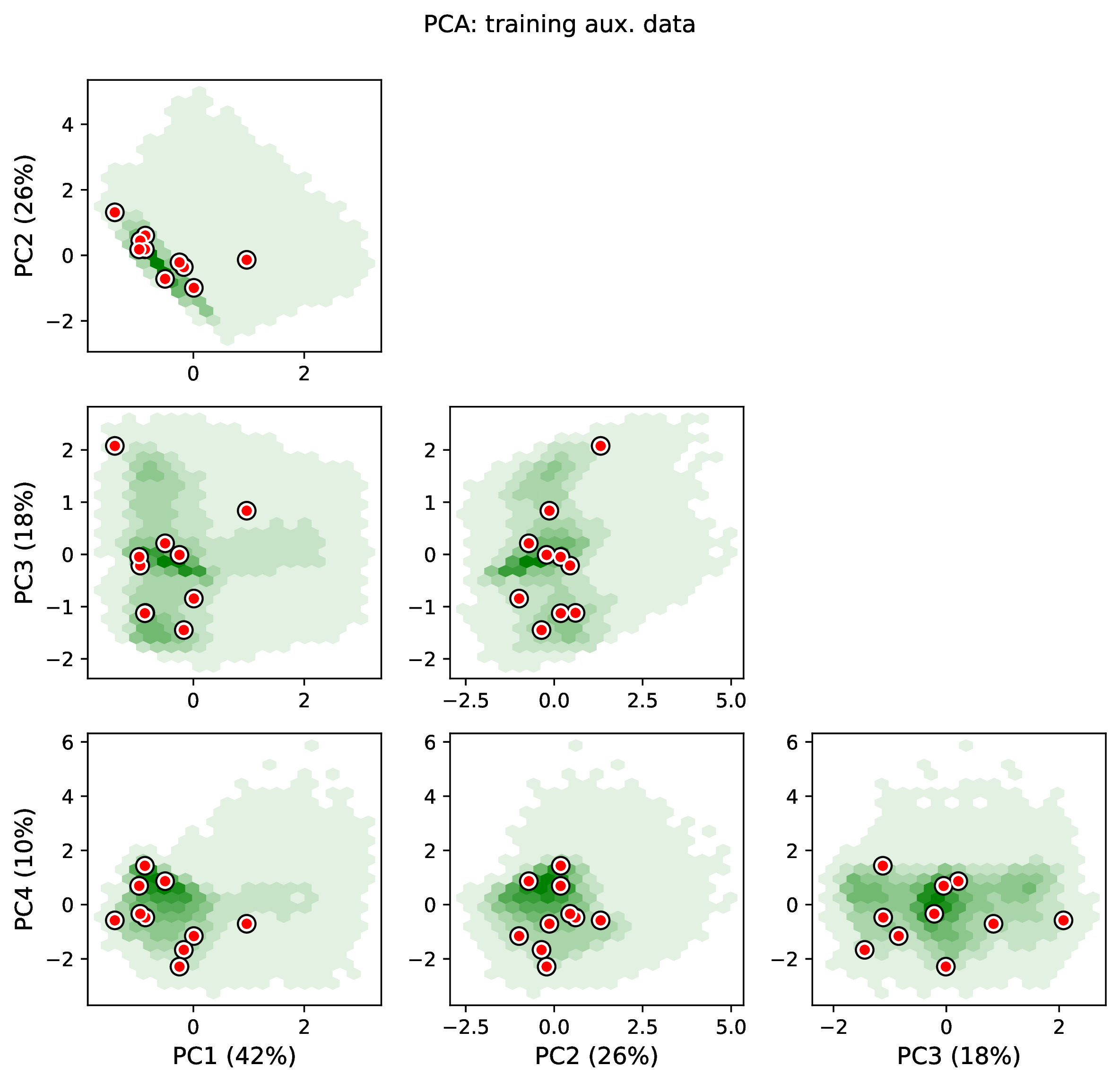
Plot collects all results from the Format, Train, and Estimate steps to compile a set of useful figures, listed below. When results from Estimate are available, the step will integrate it into other figures to contextualize where that input dataset and estimated labels fall with respect to the training dataset.

Importantly, Plot will report instances where training, test, and empirical input datasets and output estimates are unusually different. This informs users of poor network behavior (see Safe Usage).

Plots are stored within plot_dir. Colors for plot elements can be modified with plot_train_color, plot_label_color, plot_test_color, plot_val_color, plot_aux_color, and plot_est_color using hex codes or common color names supported by Matplotlib.

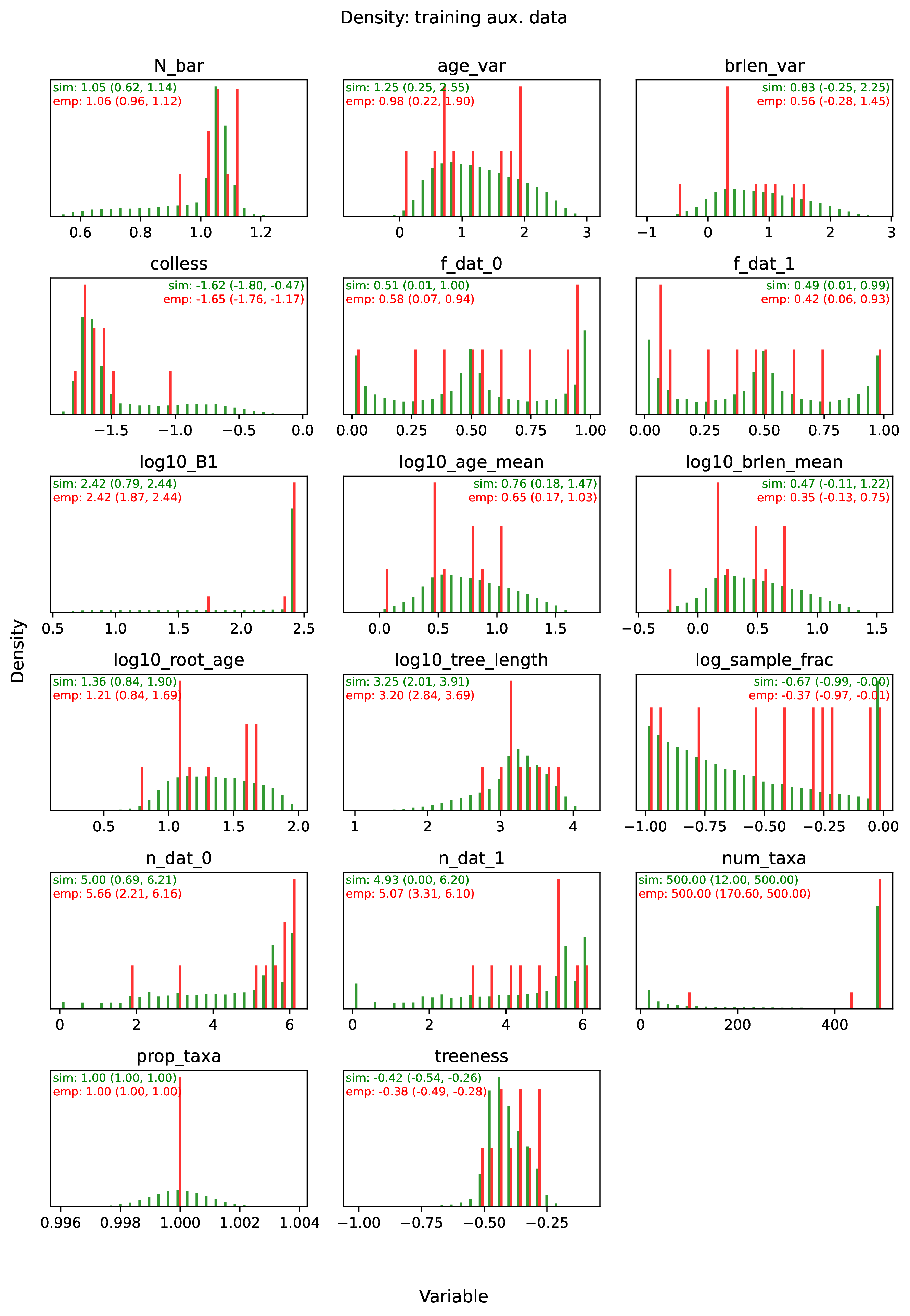
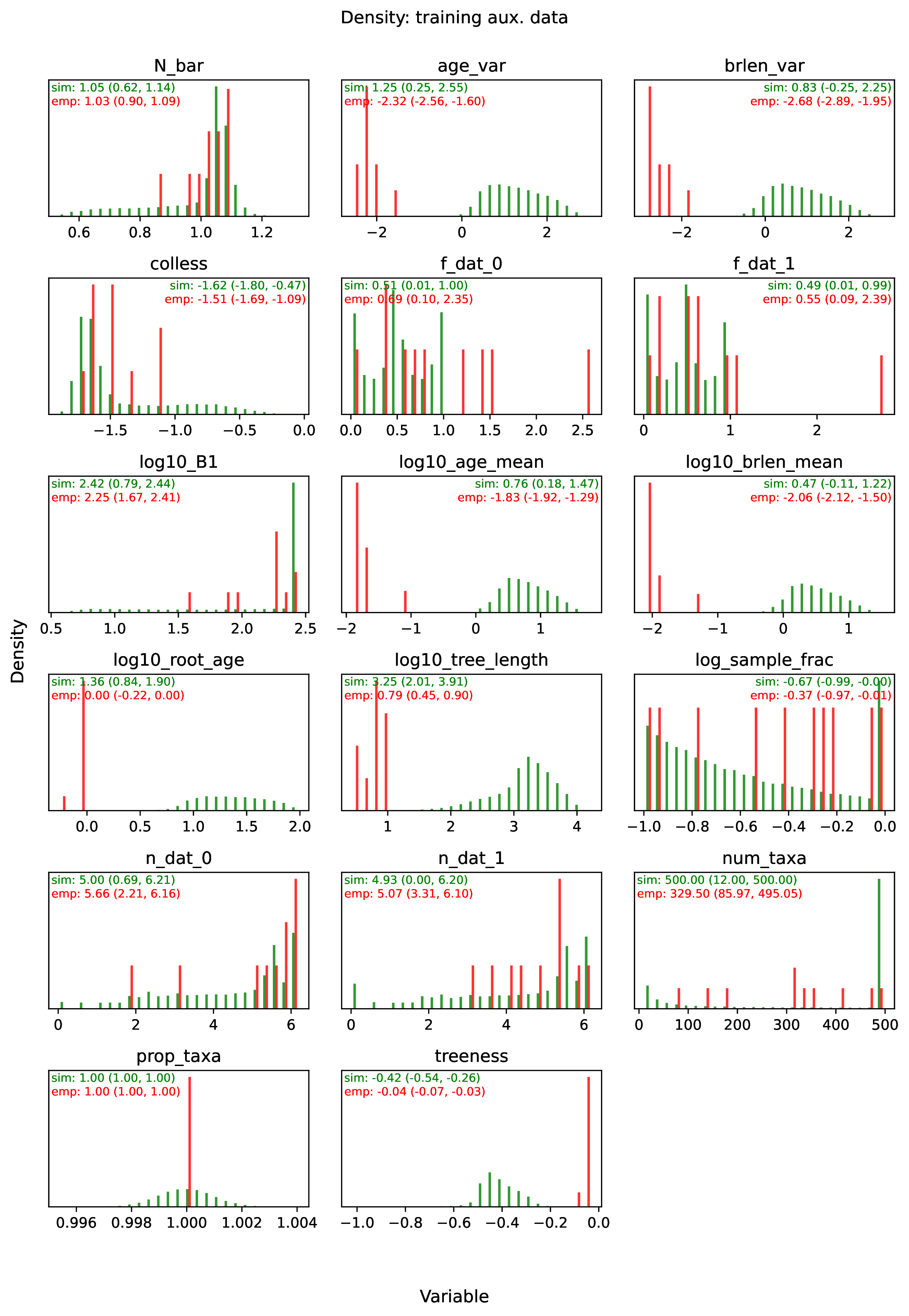
• summary.pdf contains all figures in a single plot

• summary.csv records important results in plain text format

• density_<dataset_name>_aux_data.pdf - densities of all values in the auxiliary dataset; red line for empirical dataset; run for training and empirical datasets

• density_<dataset_name>_label.pdf - densities of all values in the auxiliary dataset; red line for empirical dataset; run for training and empirical datasets

• pca_<dataset_name>_aux_data.pdf - pairwise PCA of all values in the auxiliary dataset; red dot for empirical dataset; run for training and empirical datasets

• pca_<dataset_name>_label.pdf - pairwise PCA of all values in the auxiliary dataset; red dot for empirical dataset; run for training and empirical datasets

• train_history.pdf - loss performance across epochs for test/validation datasets for entire network

• <dataset_name>_estimate_<num_label_name>.pdf - point estimates and calibrated estimation intervals of numerical parameters for test or training datasets

• <dataset_name>_estimate_<cat_label_name>.pdf - confusion matrix of categorical parameters for test or training dataset

• empirical_estimate_num_<N>.pdf - simple plot of point estimates and calibrated prediction intervals for each empirical dataset

• empirical_estimate_cat_<N>.pdf - simple bar plot for each empirical dataset

• network_architecture.pdf - visualization of Tensorflow architecture

The Tutorial and Safe Usage pages display examples of figures and explain how to interpret them.

Workspace

This section describes how phyddle organizes files and directories in its workspace.

Note

We strongly recommend that beginning users follow this general workspace filesystem design. Advanced users should find it is easy to customize locations for config files, simulation scripts, and output directories.

We recommend using the default directory structure for new projects to simplify project management. By default, dir is set to ./ and prefix is set to out. Output for each step is then stored in a subdirectory named after the step and beginning with the appropriate prefix.

For example, results from Simulate are stored in the simulate subdirectory of the dir` directory. If the sim_dir setting is provided, Simulate results are stored into that exact directory. For example, if dir is set to the local directory ./, then Simulate results are saved to ./simulate. If sim_dir is set to ../new_project/new_simulations then Simulate results are stored there regardless of the dir setting.

Similarly, if prefix is set to out, then all simulated datasets begin with the prefix out. If the setting sim_prefix is set to sim, then files generated by Simulate begin with the prefix sim.

Briefly, the workspace directory of a typical phyddle project contains two important files

• config.py that specifies default settings for phyddle analyses in this project

• sim_one.R (or a similar name) that defines a valid simulation script

and seven subdirectories for the pipeline analysis

• simulate contains raw data generated by simulation

• format contains data formatted into tensors for training networks

• train contains trained networks and diagnostics

• estimate contains new test datasets their estimations

• plot contains figures of training and validation procedures

• empirical contains raw data for your empirical analysis

• log contains runtime logs for a phyddle project

This section will assume all steps are using the example project bundled with phyddle was generated using the command phyddle --make_cfg.

phyddle -c ./workspace/example/config.py --end_idx 25000

This corresponds to a 3-region equal-rates GeoSSE model. All directories have the complete file set, except ./simulate contains only 20 original examples.

A standard configuration for a project named example would store pipeline work into these directories:

./simulate       # output of Simulate step
./empirical      # your empirical dataset
./format         # output of Format step
./train          # output of Train step
./estimate       # output of Estimate step
./plot           # output of Plot step
./log            # logs for phyddle analyses

Soon, we give an overview of the standard files and formats corresponding to each pipeline directory. First, we describe a commands that help with workspace management.

You can easily save and share your project workspace with the following command:

cd workspace/example                         # current directory is root of
                                             #     example project directory

phyddle --save_proj example_lite.tar.gz      # save project workspace, but
                                             #     skip simulated training data
                                         #     (faster, smaller)

The resulting zip file (tarball) will contain the config file, the simulation script, and all workspace directories for pipeline steps. Note, the raw and formatted simulated training example datasets tend to be very large, and require substantial time and storage to archive, so they are not fully saved by default. To fully save all workspace project data, add the following options:

phyddle --save_proj example_full.tar.gz \    # save full project, and
        --save_train_fmt T \                 #     include simulated training data
        --save_num_sim 1000000               #     (slower, larger)

If you share the project with a collaborator or save it on a server, you can load the project for use with the command:

mkdir -p ~/new_workspace/new_project         # create new project directory
cd ~/new_workspace/new_project               # enter new project directory
phyddle --load_proj example_lite.tar.gz      # load project in directory
phyddle -s S --sim_more 10000                # (e.g.) simulate 10,000 training examples

Lastly, you can quickly remove all existing workspace directories, while preserving the config file and simulation scripts, with the following command:

cd workspace/example                         # enter directory to clean
phyddle --clean_proj                         # remove all local workspace directories

These are powerful commands, so be careful when using them. They can remove or overwrite files that you want to keep. Master these commands in a safe test directory before applying them to important workspace projects.

simulate

The Simulate step generates raw data from a simulating model that cannot yet be fed to the neural network for training. A typical simulation will produce the following files

./sim.0.tre              # tree file
./sim.0.dat.csv          # data file
./sim.0.labels.csv       # data-generating params

Each tree file contains a simple Newick string. Each data file contains state data either in Nexus format (.dat.nex) or simple comma-separated value format (.dat.csv) depending on the setting for char_format.

format

Applying Format to a directory of simulated datasets will output tensors containing the entire set of training examples, stored to, e.g. ./format. If the tensor_format setting is 'csv' (Comma-Separated Value, or CSV format), the formatted files are:

./out.empirical.phy_data.csv
./out.empirical.aux_data.csv
./out.empirical.labels.csv
./out.test.phy_data.csv
./out.test.aux_data.csv
./out.test.labels.csv
./out.train.phy_data.csv
./out.train.aux_data.csv
./out.train.labels.csv

where the phy_data.csv files contain one flattened Compact Phylogenetic Vector + States (CPV+S) entry per row, the aux_data.csv files contain one vector of auxiliary data (summary statistics and known parameters) values per row, and labels.csv contains one vector of label (estimated parameters) per row. Each row for each of the CSV files will correspond to a single, matched simulated training example. All files are stored in standard comma-separated value format, making them easily read by standard CSV-reading functions.

If the tensor_format setting is 'hdf5', the resulting files are:

./out.test.hdf5
./out.train.hdf5
./out.empirical.hdf5

where each HDF5 file contains all phylogenetic-state (CPV+S) data, auxiliary data, and label data. Individual simulated training examples share the same set of ordered examples across three internal datasets stored in the file. HDF5 format is not as easily readable as CSV format. However, phyddle uses gzip to automatically (de)compress records, which often leads to files that are over twenty times smaller than equivalent uncompressed CSV formatted tensors.

train

Training a network creates the following files in the workspace/example/train directory:

./out.cpi_adjustments.csv
./out.train_aux_data_norm.csv
./out.train_est.labels_cat.csv
./out.train_est.labels_num.csv
./out.train_history.csv
./out.train_label_est_nocalib.csv
./out.train_label_norm.csv
./out.train_true.labels_cat.csv
./out.train_true.labels_num.csv
./out.trained_model.pkl

Descriptions of the files are as follows, with the prefix omitted for brevity: * trained_model.pkl: a saved file containing the trained PyTorch model * train_label_norm.csv and train_aux_data_norm.csv: the location-scale values from the training dataset to (de)normalize the labels and auxiliary data from any dataset * train_true.labels.csv: the true values of labels for the training and test datasets, where columns correspond to estimated labels (e.g. model parameters) * train_est.labels.csv: the trained network estimates of labels for the training and test datasets, with calibrated prediction intervals, where columns correspond to point estimates and estimates for lower CPI and upper CPI bounds for each named label (e.g. model parameter) * train_label_est_nocalib.csv: the trained network estimates of labels for the training and test datasets, with uncalibrated prediction intervals * train_history.csv: the metrics across training epochs monitored during network training * cpi_adjustments.csv: calibrated prediction interval adjustments, where columns correspond to parameters, the first row contains lower bound adjustments, and the second row contains upper bound adjustments

estimate

The Estimate step will load empirical and simulated test datasets generated by the Format step, and then make new predictions using the network trained during the Train step. Estimation will produce the following estimates, so long as the formatted input datasets can be opened in the filesystem:

./out.empirical_est.labels_num.csv   # output: estimated labels for empirical data
./out.empirical_est.labels_cat.csv   # output: estimated labels for empirical data
./out.test_est.labels_cat.csv            # output: estimated labels for test data
./out.test_est.labels_num.csv            # output: estimated labels for test data
./out.test_true.labels_cat.csv           # output: true labels for test data
./out.test_true.labels_num.csv           # output: true labels for test data

The out.empirical_est_labels.csv and out.test_est.labels.csv files report the point estimates and lower and upper calibrated prediction intervals (CPIs) for all parameters targeted by the param_est setting. Estimates for parameters appear across columns, where columns are grouped first by label (e.g. parameter) and then statistic (e.g. value, lower-bound, upper-bound). For example:

$ cat out.empirical_est.labels.csv
w_0_value,w_0_lower,w_0_upper,e_0_value,e_0_lower,e_0_upper,d_0_1_value,d_0_1_lower,d_0_1_upper,b_0_1_value,b_0_1_lower,b_0_1_upper
0.2867125345651129,0.1937433853918723,0.45733220552078013,0.02445545359384659,0.002880695707341881,0.10404499205878459,0.4502031713887769,0.1966340488593367,0.5147956690178682,0.06199703190510973,0.0015074254823161301,0.27544015163806645

The test_est.labels.csv and test_true.labels.csv files contain estimated and true label values for the simulated test dataset that were left aside during training. It is crucial that estimation accuracy against the test dataset is not used to inform the training process. If you view the test results and use it to modify Train settings, you should first randomly re-sample the training and test datasets from the Format step. This helps prevent overfitting and ensures that the test dataset is truly independent of the training procedure.

plot

The Plot step generates visualizations for results previously generated by Format, Train, and (when available) Estimate.

./out.empirical_estimate_cat_{i}.pdf  # categorical estimates for empirical data
./out.empirical_estimate_num_{i}.pdf  # numerical estimates for empirical data
./out.test_estimate_{param}           # estimation accuracy for test dataset
./out.train_estimate_{param}          # estimation accuracy for training dataset
./out.train_density_aux_data.pdf      # aux. data densities from Simulate/Format steps
./out.train_density_labels.pdf        # label densities from Simulate/Format steps
./out.train_pca_labels_num.pdf        # label PCA of Simulate/Format steps
./out.train_aux_data.pdf              # aux. data PCA of Simulate/Format steps
./out.train_history_{stat}.pdf        # training history for entire network
./out.network_architecture.pdf        # neural network architecture
./out.summary.pdf                     # compiled report with all figures
./out.summary.csv                     # compiled text file with numerical results

The Tutorial and Safe Usage pages display examples of figures and explain how to interpret them.

empirical

The empirical directory is used to store raw data for empirical analyses. The network from Train is only trained to make accurate predictions for datasets with the same format as the simulate directory. That means empirical datasets must have the same file types and formats as entries in the simulate directory. One difference is that empirical labels.csv files will only contain entries for “known” parameters, as specified by param_data in the configuration; they will not contain the “unknown” parameters to be estimated, specified by param_est.

./empirical/viburnum.0.tre         # tree file
./empirical/viburnum.0.dat.csv     # data file
./empirical/viburnum.0.labels.csv  # data-generating params

log

The log directory contains logs for each phyddle analysis. Log files are named according to the date and time of the analysis, and contain runtime information that may be useful for debugging or reproducing results.

Visit Overview to learn more about the files.

Formats

This page describes different internal datatype formats and file formats used by phyddle.

Input datasets

phyddle can make phylogenetic model predictions against input datasets with previously trained networks. Valid phyddle input datasets contain a set of files with a shared filename prefix. For example, a dataset with the prefix out.3 would contain a tree file out.0.tre, a character matrix file out.3.dat.nex, and (when applicable) a ‘known parameters’ file out.3.labels.csv. Simulated training datasets and real biological datasets follow the same format.

Trees are encoded as raw data in simple Newick format. Trees are assumed to be rooted, bifurcating, time-calibrated trees. Trees may be ultrametric or non-ultrametric trees. Ultrametric trees should only be analyzed using treetype == ‘extant’. Non-ultrametric trees, such as those containing serially sampled viruses or fossils should be analyzed using treetype == ‘serial’. Here is an example of an extant tree with N=8 taxa.

$ cat ./simulate/out.0.tre
((((1:0.35994691486501296,2:0.35994691486501296):1.389952711060852,(3:1.5810568349100933,(4:0.5830569936279364,5:0.5830569936279364):0.9979998412821569):0.1688427910157717):5.655066077200624,6:7.404965703126489):0.3108578683347094,(7:0.7564319839861859,8:0.7564319839861859):6.959391587475013):2.2841764285388018;

Character data may be encoded in Nexus format (char_format = ‘nex’). Here is an example of a matrix with N=8 taxa and M=3 binary characters.

$ cat ./simulate/out.0.dat.nex
#NEXUS
Begin DATA;
Dimensions NTAX=8 NCHAR=3
Format MISSING=? GAP=- DATATYPE=STANDARD SYMBOLS="01";
Matrix
    1  001
    2  010
    3  100
    4  100
    5  001
    6  001
    7  100
    8  010
;
END;

Character data may also be encoded in csv format (char_format = ‘csv’). For example:

$ cat ./simulate/out.0.dat.nex
1,0,0,1
2,0,1,0
3,1,0,0
4,1,0,0
5,0,0,1
6,0,0,1
7,1,0,0
8,0,1,0

Some models will accept “known” data-generating parameters as input. For example, if not all taxa were included in the phylogeny, a model might accept a sampling fraction label as input. Any labels that are marked under the param_data setting will be encoded into the auxiliary data tensor during formatting. Example:

$ cat ./simulate/out.0.labels.csv
birth_1,birth_2,death,state_rate,sample_frac
0.5728,0.9082,0.1155,0.0372,0.1114

where the setting param_data == ['sample_frac'] would ensure that only the sample_frac entry is included in auxiliary data.

Tensor formats

Phylogenetic data (e.g. from a Newick file) and character matrix data (e.g. from a Nexus file) are encoded into compact phylogenetic state tensors. Internally, phyddle uses `dendropy.Tree` to represent phylogenies, pandas.DataFrame to represent character matrices (verify), and numpy.ndarray to store phylogenetic-state tensors.

There are two types of phylogenetic-state tensors in phyddle: the compact bijective ladderized vector + states (CBLV+S) and the compact diversity vector + states (CDV+S). CBLV+S is used for trees that contain serially sampled (non-ultrametric) taxa whereas CDV+S is used for trees that contain only extant (ultrametric) taxa. The tree_width of the encoding defines the maximum number of taxa the phylogenetic-state tensor may contain. The tree_encode setting determines if the tree is a 'serial' tree encoded with CBLV+S or an 'extant' tree encoded with CDV+S. Setting brlen_encode and char_encode alter how information is stored into the phylogenetic-state tensor.

CBLV+S

This is an example for the CBLV+S encoding of 5 taxa with 2 characters. This is the Newick string:

(((A:2,B:1):1,(C:3,D:2):3):1,E:2);

This is the Nexus file:

#NEXUS
Begin DATA;
Dimensions NTAX=5 NCHAR=2
Format MISSING=? GAP=- DATATYPE=STANDARD SYMBOLS="01";
Matrix
    A  01
    B  11
    C  10
    D  10
    E  01
;
END;

These data can be encoded in different ways, based on the char_encode setting. When char_encode == 'integer' then the encoding will treat each character as a row in the resulting data matrix, and assign the appropriate integer-valued state to that character for each taxon. Alternatively, when char_encode == 'one_hot' then the encoding will treat every distinct state-character combination as its own row in the resulting data matrix, then mark each species as 1 for a cell when a species has that character-state and 0 if not. One-hot encoding is applied individually to each homologous character (fewer distinct combinations) not against the entire character set (more distinct combinations).

Ladderizing clades by maximum root-to-tip distance orders the taxa C, D, A, B, then E, which correspond to the first five entries of the CBLV+S tensor. When brlen_encode is set to 'height_only' the un-rescaled CBLV+S file would look like this:

# NOTE: The CBLV+S tensor is shown in this orientation for readability.
#       phyddle stores the tensor as the transpose of this in memory,
#       meaning rows correspond to taxa, and columns correspond to branch
#       length information.

# C,D,A,B,E,-,-,-,-,-
  7,2,3,1,2,0,0,0,0,0  # tip-to-node distance
  0,4,1,2,0,0,0,0,0,0  # node-to-root distance
  1,1,0,1,0,0,0,0,0,0  # character 1
  0,0,1,1,1,0,0,0,0,0  # character 2

and like this when brlen_encode is set to 'height_brlen':

# C,D,A,B,E,-,-,-,-,-
  7,2,3,1,2,0,0,0,0,0  # tip-to-node distance
  0,4,1,2,0,0,0,0,0,0  # node-to-root distance
  3,2,2,1,2,0,0,0,0,0  # tip edge length
  0,3,1,1,0,0,0,0,0,0  # node edge length
  1,1,0,1,0,0,0,0,0,0  # character 1
  0,0,1,1,1,0,0,0,0,0  # character 2

By default, all branch length entries are rescaled from 0 to 1 as proportion to tree height (formatted to ease reading):

#    C,   D,   A,   B,   E,   -,   -,   -,   -,   -
  1.00,0.29,0.43,0.14,0.29,   0,   0,   0,   0,   0  # tip-to-node distance
  0.00,0.57,0.14,0.29,0.00,   0,   0,   0,   0,   0  # node-to-root distance
  0.43,0.29,0.29,0.14,0.29,   0,   0,   0,   0,   0  # tip edge length
  0.00,0.43,0.14,0.14,0.00,   0,   0,   0,   0,   0  # node edge length
     1,   1,   0,   1,   0,   0,   0,   0,   0,   0  # character 1
     0,   0,   1,   1,   1,   0,   0,   0,   0,   0  # character 2

CDV+S

CDV+S is used to encode phylogenetic-state information for trees of only extant taxa. CDV+S has a similar structure to CBLV+S, except in two principal ways. First, CDV+S uses total subclade diversity rather than tip node with max distance-from-root-node to determine how to ladderize the tree, which in turn determines which columns are associated with which tip nodes. Second, because CDV+S is used for extant-only trees, it does not need to report the redundant information about tip-to-node distances, as the tip-to-root distances are equal among all tips (by definition). This means that CDV+S does not contain a row with tip-to-node distances (the first row of CBLV+S).

For example, the following Newick string for an ultrametric tree

(((A:5,B:5):1,(C:3,D:3):3):1,E:7);

and associating the same character data as above with taxa A through E yields the following CDV+S tensor:

# NOTE: The CDV+S tensor is shown in this orientation for readability.
#       phyddle stores the tensor as the transpose of this in memory,
#       meaning rows correspond to taxa, and columns correspond to branch
#       length information.

# C,D,A,B,E,-,-,-,-,-
  0,4,1,2,0,0,0,0,0,0  # node-to-root distance
  3,2,2,1,2,0,0,0,0,0  # tip edge length
  0,3,1,1,0,0,0,0,0,0  # node edge length
  1,1,0,1,0,0,0,0,0,0  # character 1
  0,0,1,1,1,0,0,0,0,0  # character 2

Auxiliary data

The auxiliary data tensor contains a panel of summary statistics extracted from the inputted phylogeny and character data matrix for a given dataset. Currently, phyddle generates the following summary statistics:

tree_length       # sum of branch lengths
num_taxa          # number of terminal taxa in tree/data
root_age          # longest root-to-tip distance
brlen_mean        # mean of branch lengths
brlen_var         # variance of branch lengths
brlen_skew        # skewness of branch lengths
age_mean          # mean of internal node ages
age_var           # variance of internal node ages
age_skew          # skewness of internal node ages
B1                # B1 tree measure (Dendropy)
N_bar             # N_bar tree measure (Dendropy)
colless           # Colless tree measure (Dendropy)
treeness          # treeness measure (Dendropy)
f_dat_0           # frequency of taxa with character in state 0
f_dat_1           # frequency of taxa with character in state 1
...

The auxiliary data tensor also contains any parameter values that shape the data-generating process, but can be treated as “known” rather than needing to be estimated. For example, the epidemiologists may assume they know the rate of infection recovery (gamma) based on public health or clinical data. Parameters may be treated as data by providing the labels for those parameters in the param_data entry of the config file. For example, setting 'param_data' : [ 'sample_frac' ] could be used to inform phyddle that the recovery rate and susceptible population sizes for location 0 are known for a phylogenetic SIR analysis.

Safe Usage

We designed phyddle to be user-friendly. However, we caution users that deep learning approaches can easily produce nonsensical and/or misleading results when irresponsibly. Below, we describe several issues that newcomers to deep learning might encounter, along with how to diagnose and solve them.

Poor accuracy or coverage

Neural networks are trained to make accurate predictions, such as point estimates and prediction intervals. Poor accuracy or coverage is a common problem and easily detected, but it can arise for many reasons.

To diagnose poor accuracy or coverage, run the Plot step. Review the scatter plots of true versus estimated labels for the Train and Test datasets. Accurate predictions for numerical labels should fall along the 1:1 line, with a slope close to 1.0. Coverage levels should be close to the target level. For categorical variables, the confusion matrix should show high values along the diagonal and small values elsewhere. phyddle will print warnings if accuracy or coverage is poor in the Training or Test datasets.

To correct the issue, undertraining, overtraining, small training datasets, poor network architecture, or other issues may be at play. The following sections provide ideas to fix the issue.

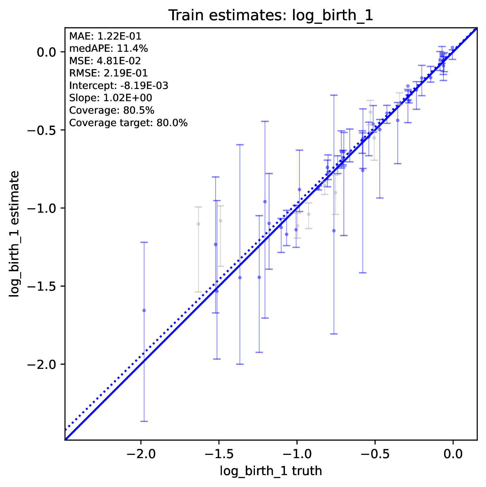Accurate numerical estimates

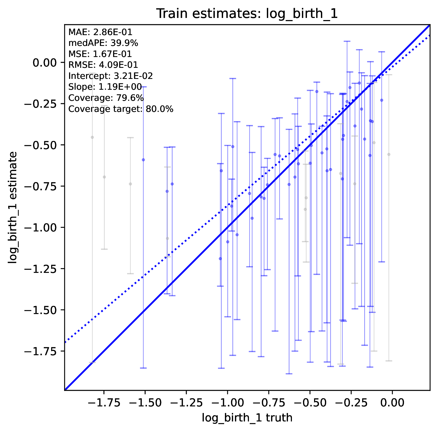Inaccurate numerical estimates

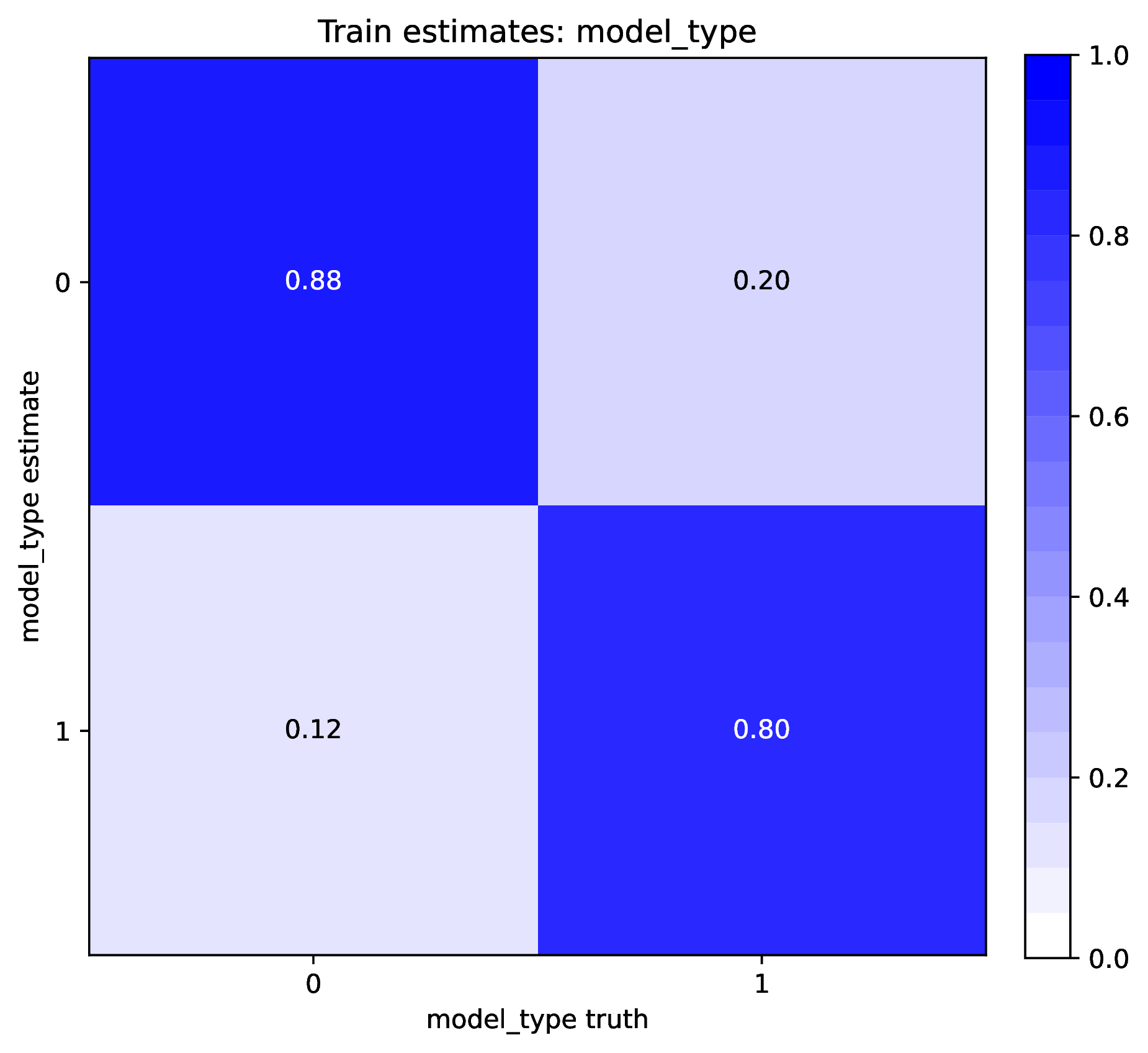Accurate categorical estimates

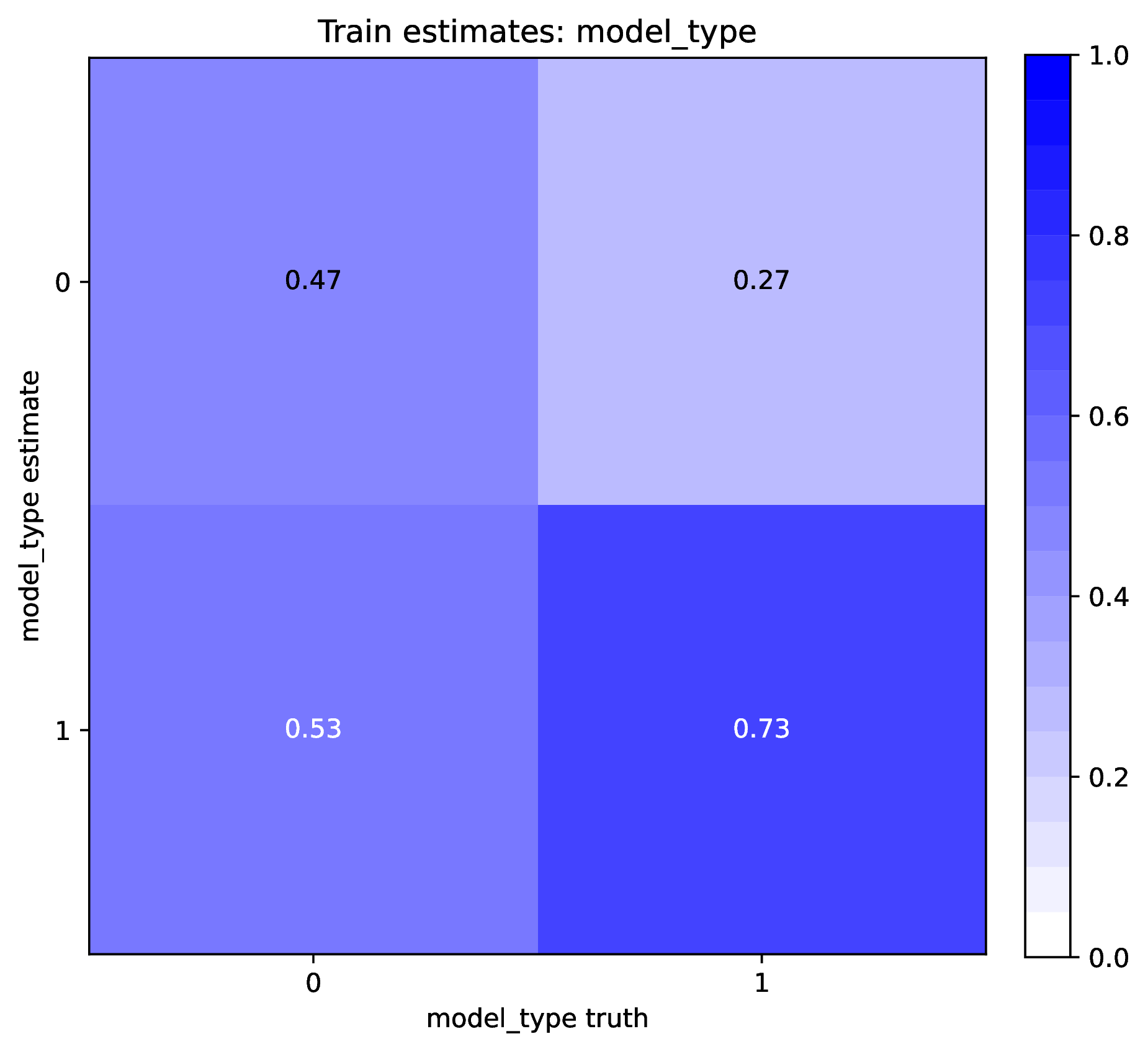Inaccurate categorical estimates

Undertraining and overtraining

The loss score for the training dataset will typically decrease as the number of training epochs increases. This is because typically neural networks have thousands of weight and bias parameters to adjust, and small adjustments can easily squeeze at marginal improvements to the loss score.

An undertrained network will not make accurate predictions for training, test, or validation datasets. This is because the optimizer was not able to learn the optimal network parameters before training concluded. On the other hand, an overtrained network will only make accurate predictions for the training dataset, while making inaccurate predictions against non-training datasets, such as the test and validation datasets.

To diagnose undertraining problems, review the training history plot. If the loss score for both the training and validation datasets is still decreasing by the end of the training period, then the network is undertrained.

To correct for undertraining, double the number of training epochs or use larger batch sizes of training examples.

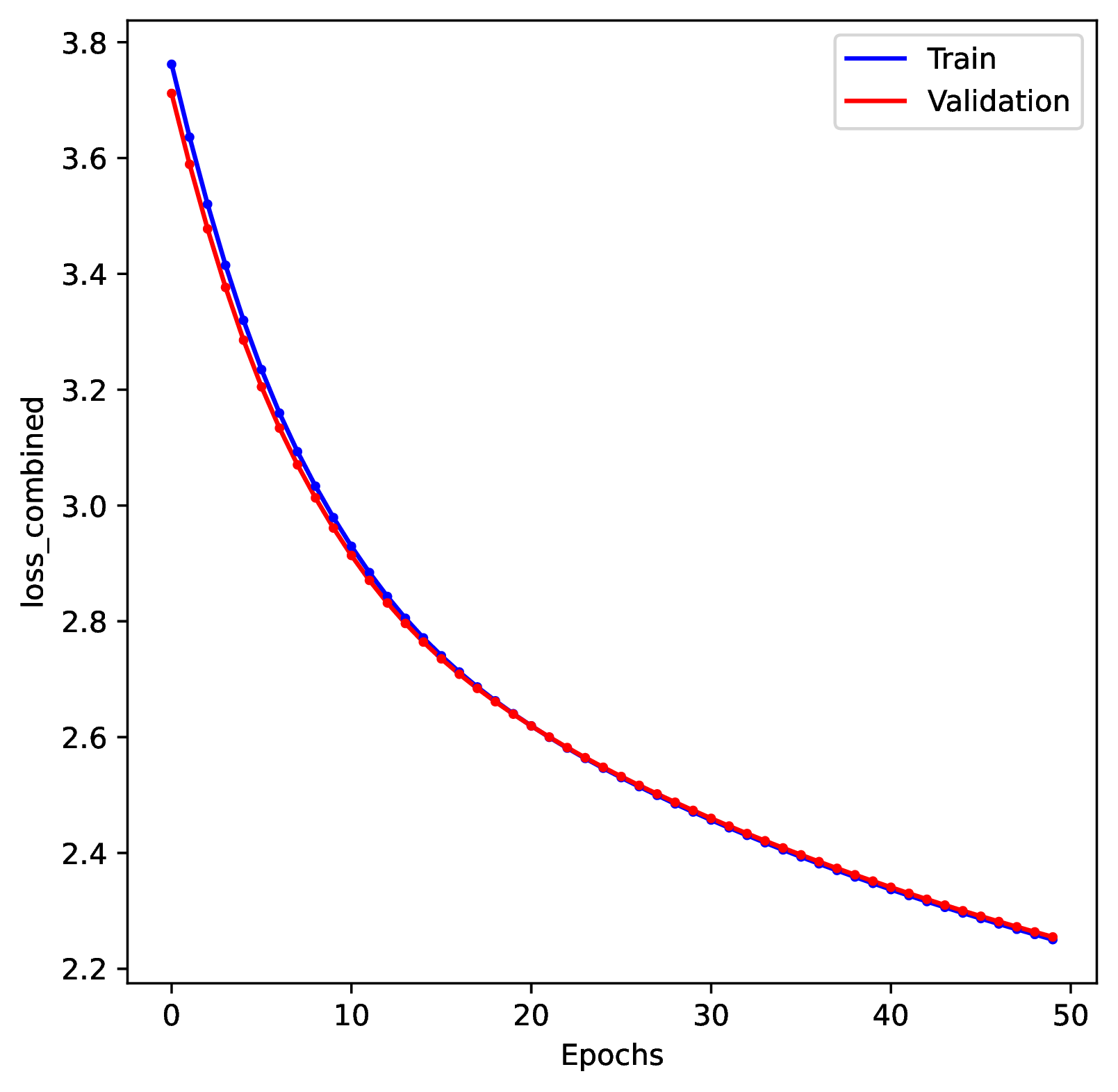
To diagnose overtraining problems, run the Plot step. Review the training history plot. If you see that the loss score for the training dataset continuously decreases while the loss score for the validation dataset increases (making a ‘U’ shape) then the network is overtrained.

To correct for overtraining, you can either specify a shorter number of training epochs, decrease the training batch sizes, or use stronger early stopping rules. To prevent overtraining, the default behavior in phyddle is to stop training when the validation loss score increases for 3 consecutive epochs.

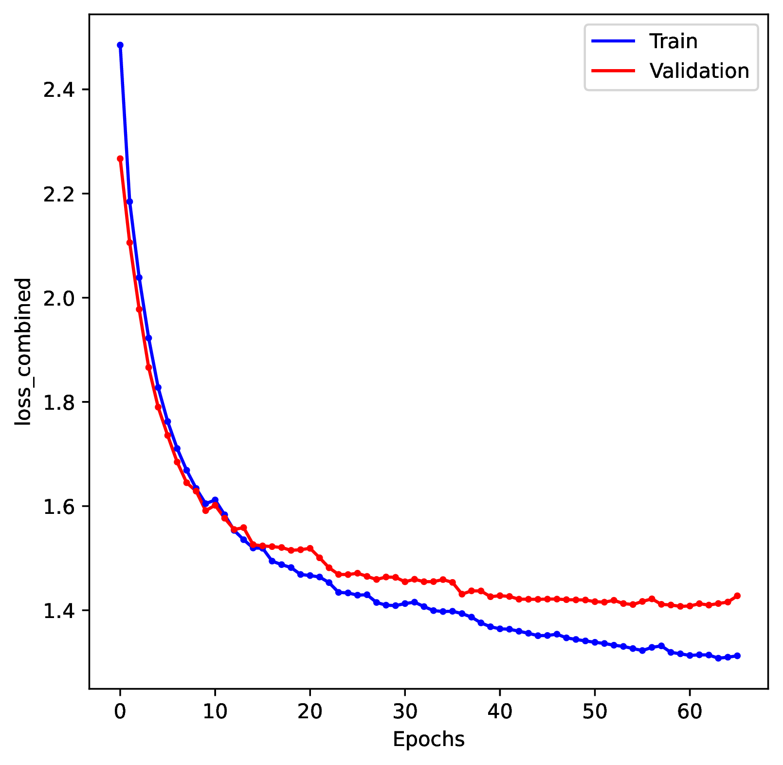Good training

Undertraining

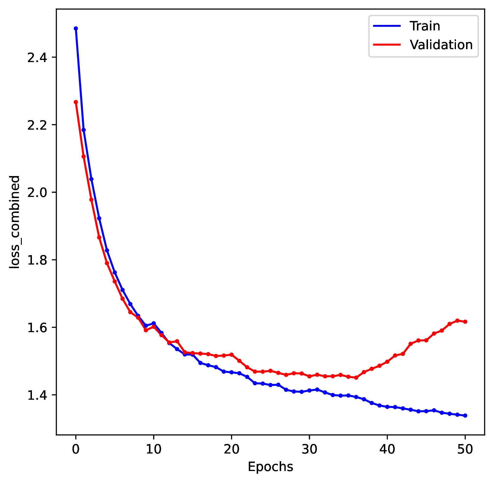Overtraining

Small training datasets

Supervised learning requires large training datasets to train networks to perform accurately. Most of the workspace examples are designed to work well with ~50,0000 training examples. Small training datasets do not contain enough examples to densly represent general relationships between input and output patterns. In this case, the trained network will have poor prediction accuracy against the training, test, and validation datasets – even if the network was trained to its optimal level.

To diagnose this issue, run the Plot step. Verify that the training history plot does not show evidence for overtraining or undertraining. Next, verify the network has poor prediction accuracy for the training and test datasets.

To fix the issue, simulate twice as many datasets, retrain the network, and then assess whether accuracy improved. If it does, continue simulating data until prediction accuracy for the training and test datasets stabilizes.

Suboptimal network size

Neural networks are composed of layers of nodes that are interconnected through series of activation functions that are optimized during training. In general, increasing network depth (more layers) and width (more nodes) allows a network to easily express a broader variety of relationships between inputs and outputs (higher capacity), which can increase accuracy when properly trained. However, because larger networks have more parameters to optimize, they are also prone to overtraining.

To diagnose issues with network size, run the Plot step. If the network is too small, the network will underperform across all prediction tasks. The training history plot will show rapid convergence towards the optimal loss score, but the final loss score will be higher than expected. In addition, prediction accuracy for the training and test datasets will be in agreement. If the network is too large, then the training history will show evidence of overtraining, and the prediction accuracy for the training dataset will be high, with degraded accuracy for the test dataset.

To fix the issue, compare the prediction accuracy of networks trained with different depths and widths. To do this, modify the numbers of layers and nodes through the configuration file, train the new network, and compare differences in accuracy and training time with other network designs.

Out-of-distribution examples

Supervised learning uses large datasets, composed of pairs of input (features) and output (labels), to train neural networks to accurately predict labels from new datasets. Properly trained network should perform well at making predictions for inputs similar to those in the training dataset. For example, the training, test, validation, and calibration examples are all samples from the same distribution of data (i.e. through the model-based simulator). New empirical datasets might look like these data (in-distribution) or they might look radically different (out-of-distribution). Out-of-distribution examples are do not resemble any training examples, so the network cannot be trusted to make accurate predictions from them.

To diagnose this issue, run the Estimate and Plot steps. The Estimate step will report any empirical datasets and variables that are outliers with respect to the training dataset. The Plot step will generate PCA plots and histograms of variables for the training and empirical datasets; inspect the plots to identify empirical examples that are outliers.

To solve the problem, verify the empirical datasets are formatted in the same way as the training dataset. For example, make sure phylogenetic branch lengths and traits are measured in the same units, and that discrete trait labels use the same encoding. If they are formatted correctly, then you will need to simulate a new and more-variable training dataset that will include the range of expected input and output variables from the empirical data. For example, if your empirical trees are roughly 20 to 50 million years in height, consider simulating training trees that are between 5 and 100 million years in height.

Within-distribution

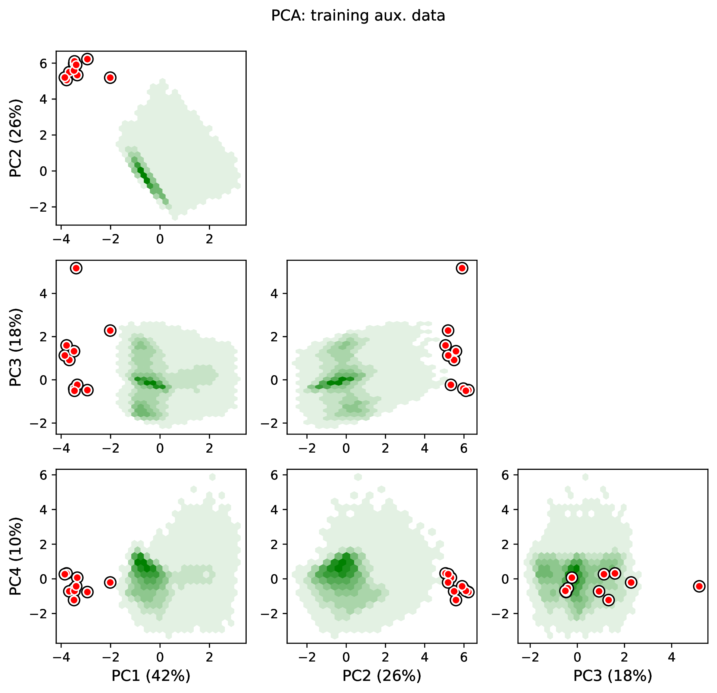Out-of-distribution

Within-distribution

Out-of-distribution

Simulator errors

phyddle uses simulated examples to train neural networks. This means that the quality of the training data is only as good as the simulator that generates it. Untested simulators often contain coding or mathematical errors. We stress that if the simulator generates erroneous datasets, then the network will be trained to confidently make erroneous predictions!

Diagnosing the issue is not easy. A network trained on a bad simulator will still make accurate predictions for the training, test, and validation datasets. However, predictions for empirical datasets will remain bad despite attempts to adjust the size or variability of training examples, network architecture, or training settings.

Use other simulators, estimation methods, and theory to validate the correctness of your simulator. One good option is to find a special case of your model that is identical to a second more-tractable model: e.g. reduce your time-heterogeneous SSE model to a pure birth process. In these cases, you can compare the output of your simulator to the output from a second peer-reviewed simulator. Simulate data with both simulators under the same model conditions, and verify they produce similar distributions of output: e.g. both simulators yield trees with similar tree height distributions. Another option is to use or derive theory to verify that your simulator produces the expected output: e.g. show your simulator generates the correct expected number of species for a given set of parameters and duration of evolutionary time. In cases where your model has a tractable likelihood, the estimates of your trained network should agree with those from a likelihood-based estimator. Likelihood-based Bayesian coverage experiments for extremely small datasets (e.g. 3 species, 2 characters) are sufficient to show the simulator is correct.

Unintended signal

Neural networks are designed to learn patterns from data, which means they can also learn unintended patterns. In particular, phyddle networks are only expected to make accurate predictions for new empirical datasets that follow the same format as the simulated datasets. Unless handled carefully by the analyst, simulated and empirical datasets might differ in terms of scale (e.g. thousands vs. billions of years for tree height), transformation (e.g. log vs. linear trait measurements), character encoding (e.g. the simulator sorts nucleotide sites by variability, but the empirical preserves its ordering), state encoding (e.g. the simulator uses state 0, but the empirical data uses state 1 to represent a widespread species in regions A and B), or other ways. While phyddle will internally rescale traits and tree heights internally to mitigate some issues, it cannot automatically correct for biases that might arise due to encodings or transformations.

To diagnose the issue, run the Estimate and Plot steps with the empirical data included. If the data representation is grossly mismatched, the issue may appear as an out-of-distribution error, and you may see that the empirical data are outliers in the PCA plots and/or histograms. Identifying the issue for subtle differences in data representation may require a deep understanding of the model and the data.

To correct the issue, you need to ensure that the empirical data are represented in the same way as the simulated data. For example, if your simulator log-transforms traits before saving the simulation to file, you must do the same for your empirical dataset. A good strategy for this is to write code for necessary data adjustments (e.g. log-transformations, shuffling character order) and that same code for both the simulated and empirical data.

Model design

There are many subtle factors related to model design that can impact the performance of estimation tasks. For example, models with non-identifiable parameters can be difficult or impossible to estimate – e.g. estimating compound parameters for evolutionary distance rather than separate parameters for rate and time. In other cases, the parameterization of the model can impact learning efficiency – e.g. using birth and death rates versus diversification and turnover parameters is known to influence how easily maximum likelihood methods estimate birth-death model parameters.

There are far too many issues related to model design to describe here. In general, it is safe to assume that deep learning methods will face similar difficulties as likelihood-based methods for standard model estimation tasks. If theory shows that a model is non-identifiable, neither method would precisely estimate all of that model’s parameters.

Designing models is complicated and benefits from mathematical expertise and experience. We recommend that biologists who are creating novel models for the first time consult with theoreticians identify potential flaws in the model design.

Nonsensical results

When applying a statistical model or inference method to analyze an empirical dataset, it’s critical to verify that the results are sensible. Models and methods cannot put the results it finds into a broader scientific context. For example, inferring a net diversification rate of 1,000 species per species per Myr for a bird clade might be an earth-shattering result that fundamentally changes our understanding of vertebrate evolution. Or perhaps the model is poorly designed. Or perhaps the simulator contained a bug. Or perhaps the network was overtrained. Or perhaps the dataset contained an error.

We urge biologists to use their knowledge of the empirical system and the model properties to interpret results. Do not hesitate to question the results of any statistical analysis, with phyddle or otherwise, especially if they cannot be explained clearly and convincingly. If you suspect your results cannot be trusted, explore whether results are robust to adjustments in the dataset or analysis settings, and to what extent the results can be replicated with other methods.

Assorted tricks

Here are a few tricks for using phyddle using a Unix-based terminal. These commands assume a standard phyddle workspace directory structure.

Make a new config file

# Create and modify new config file
phyddle --make_cfg

# Rename new config
mv config_default.py my_new_config.py

# Design new config
edit my_new_config.py

# Run using new config
phyddle -c my_new_config.py

Run a pipeline with modified command-line settings

# Run full pipeline while changing calibration and validation proportions
phyddle -c config.py --cal_prop 0.10 --val_prop 0.10

Re-run part of the pipeline with modified command-line settings

# Re-run pipeline Train, Estimate, and Plot steps with new training settings
phyddle -c config.py -s TEP --num_epoch 10 --trn_batch_size 64

Redirect input/output across pipeline steps

# Run full pipeline
phyddle -c config.py

# Re-run Train, Estimate, Plot steps with new settings, saved to other_project
phyddle -c config.py \
        -s TEP \
        --trn_dir ../other_project/train \
        --est_dir ../other_project/estimate \
        --plt_dir ../other_project/plot \
        --num_epochs 40 \
        --trn_batch_size 512

# Alternatively, point `dir` to other project point Format to this project
  phyddle -c config.py \
          -s TEP \
          --dir ../other_project \
          --fmt_dir ./format \
          --num_epochs 40 \
          --trn_batch_size 512

Process alternative empirical data using previously trained network

# Run full pipeline
phyddle -c config.py

# Format, Estimate, and Plot empirical data against trained network
phyddle -c config.py \
        -s FEP \
        --no_sim \
        --emp_dir ../other_project/empirical \
        --est_dir ./new_estimate \
        --plt_dir ./new_plot

Simulate new training examples

# Simulate training examples 0 to 999, storing results
# workspace/simulate/my_project
phyddle -s S -c config.py --start_idx 0 --end_idx 1000

# Simulate 4000 more training examples, 0 to 4999
phyddle -s S -c config.py --sim_more 4000

# Perform remaining Format, Train, Estimate, Plot steps
phyddle -s FTEP -c config.py

# ...or, to Simulate more and re-run all steps
phyddle -c config.py --sim_more 4000

Run an analysis for a tree without character data

To analyze a model that only generates trees but not character data (e.g. a birth-death process), design your simulator to write to file a character matrix with the same taxon set, but with zeroes for all character state information. When training, only the trees will contain variation that can be used to estimate model parameters. Future versions of phyddle will allow for the direct analysis of trees without character data, without needing this workaround.

Run an analysis for data without a tree

To analyze a model that only generates data but no tree (e.g. a normal distribution), design your simulator to write a two-taxon tree ((A:1,B:1);) to the tree file, a two-taxon character matrix with zeroes for states to the character matrix file (see above), and all data of actual interest into the labels file. Then, identify all variables of interst in param_data. When training, only the known parameters will contain variation that can be used to estimate model parameters. Future versions of phyddle will allow for the direct analysis of data without trees and character data, without needing this workaround.

Quick access to workspace directories from console via GUI

On Mac OS X, you can press the Option key and click a directory path to open a Finder window to that directory.

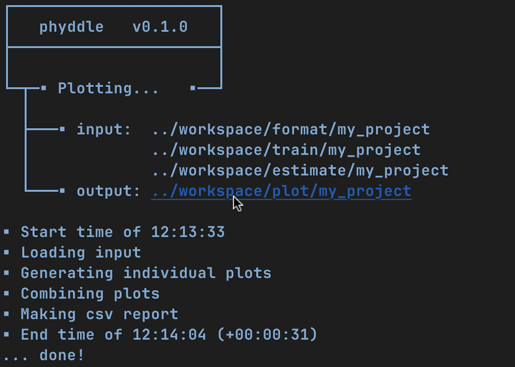
Example run

The output of phyddle pipeline analysis will resemble this:

┏━━━━━━━━━━━━━━━━━━━━━━┓
┃   phyddle   v0.1.1   ┃
┣━━━━━━━━━━━━━━━━━━━━━━┫
┃                      ┃
┗━┳━▪ Simulating... ▪━━┛
  ┃
  ┗━━━▪ output:  ./simulate

▪ Start time of 20:37:07
▪ Simulating raw data
Simulating: 100%|█████████████████████████| 100/100 [00:20<00:00,  4.94it/s]
▪ Total counts of simulated files:
  ▪ 31030 phylogeny files
  ▪ 31030 data files
  ▪ 31030 labels files
▪ End time of 20:37:31 (+00:00:24)
... done!
┃                      ┃
┗━┳━▪ Formatting... ▪━━┛
  ┃
  ┣━━━▪ input:   ./empirical
  ┃              ./simulate
  ┗━━━▪ output:  ./format

▪ Start time of 20:37:32
▪ Collecting simulated data
▪ Encoding simulated data as tensors
Encoding: 100%|██████████████████████| 31030/31030 [04:36<00:00, 112.08it/s]
Encoding found 31030 of 31030 valid examples.
▪ Splitting into train and test datasets
▪ Combining and writing simulated data as tensors
Making train hdf5 dataset: 29479 examples for tree width = 500
Making test hdf5 dataset: 1551 examples for tree width = 500
▪ Collecting empirical data
▪ Encoding empirical data as tensors
Encoding: 100%|█████████████████████████████| 10/10 [00:50<00:00,  5.08s/it]
Encoding found 10 of 10 valid examples.
▪ Combining and writing empirical data as tensors
Making empirical hdf5 dataset: 10 examples for tree width = 500
▪ End time of 20:43:21 (+00:05:49)
... done!
┗━┳━▪ Training...   ▪━━┛
  ┃
  ┣━━━▪ input:   ./format
  ┗━━━▪ output:  ./train

▪ Start time of 20:45:09
▪ Loading input:
  ▪ 22111 training examples
  ▪  5895 calibration examples
  ▪  1473 validation examples
▪ Training targets:
  ▪ log10_birth_1     [type: num]
  ▪ log10_birth_2     [type: num]
  ▪ log10_death       [type: num]
  ▪ log10_state_rate  [type: num]
▪ Building network
▪ Training network
Training epoch 1 of 10: 100%|███████████████| 44/44 [00:50<00:00,  1.14s/it]
    Train        --   loss: 1.0648
    Validation   --   loss: 0.9459

Training epoch 2 of 10: 100%|███████████████| 44/44 [00:49<00:00,  1.13s/it]
    Train        --   loss: 0.8429  abs: -0.2219  rel: -20.84%
    Validation   --   loss: 0.8125  abs: -0.1333  rel: -14.10%

Training epoch 3 of 10: 100%|███████████████| 44/44 [00:49<00:00,  1.12s/it]
    Train        --   loss: 0.7646  abs: -0.0782  rel: -9.28%
    Validation   --   loss: 0.7716  abs: -0.0410  rel: -5.04%

Training epoch 4 of 10: 100%|███████████████| 44/44 [00:49<00:00,  1.12s/it]
    Train        --   loss: 0.7218  abs: -0.0429  rel: -5.61%
    Validation   --   loss: 0.7275  abs: -0.0441  rel: -5.71%

Training epoch 5 of 10: 100%|███████████████| 44/44 [00:48<00:00,  1.11s/it]
    Train        --   loss: 0.6917  abs: -0.0300  rel: -4.16%
    Validation   --   loss: 0.6930  abs: -0.0345  rel: -4.74%

Training epoch 6 of 10: 100%|███████████████| 44/44 [00:48<00:00,  1.11s/it]
    Train        --   loss: 0.6657  abs: -0.0261  rel: -3.77%
    Validation   --   loss: 0.6874  abs: -0.0056  rel: -0.81%

Training epoch 7 of 10: 100%|███████████████| 44/44 [00:49<00:00,  1.13s/it]
    Train        --   loss: 0.6417  abs: -0.0240  rel: -3.61%
    Validation   --   loss: 0.6621  abs: -0.0253  rel: -3.68%

Training epoch 8 of 10: 100%|███████████████| 44/44 [00:50<00:00,  1.14s/it]
    Train        --   loss: 0.6264  abs: -0.0153  rel: -2.38%
    Validation   --   loss: 0.6549  abs: -0.0072  rel: -1.09%

Training epoch 9 of 10: 100%|███████████████| 44/44 [00:49<00:00,  1.13s/it]
    Train        --   loss: 0.6144  abs: -0.0119  rel: -1.91%
    Validation   --   loss: 0.6376  abs: -0.0173  rel: -2.64%

Training epoch 10 of 10: 100%|██████████████| 44/44 [00:49<00:00,  1.14s/it]
    Train        --   loss: 0.6078  abs: -0.0067  rel: -1.08%
    Validation   --   loss: 0.6307  abs: -0.0069  rel: -1.08%

▪ Processing results
▪ Saving results
▪ End time of 20:53:47 (+00:08:38)
▪ ... done!
┃                      ┃
┗━┳━▪ Estimating... ▪━━┛
  ┃
  ┣━━━▪ input:   ./format
  ┃              ./train
  ┗━━━▪ output:  ./estimate

▪ Start time of 20:53:47
▪ Estimation targets:
  ▪ log10_birth_1     [type: num]
  ▪ log10_birth_2     [type: num]
  ▪ log10_death       [type: num]
  ▪ log10_state_rate  [type: num]
▪ Loading simulated test input
▪ Making simulated test estimates
▪ Loading empirical input
▪ Making empirical estimates
▪ End time of 20:53:49 (+00:00:02)
... done!
┃                      ┃
┗━┳━▪ Plotting...   ▪━━┛
  ┃
  ┣━━━▪ input:   ./format
  ┃              ./train
  ┃              ./estimate
  ┗━━━▪ output:  ./plot

▪ Start time of 20:55:18
▪ Loading input
▪ Generating individual plots
▪ Combining plots
▪ Making csv report
▪ End time of 20:55:35 (+00:00:17)
... done!